Note
Go to the end to download the full example code
Defining a customized technology
In this example, we extend a predefined technology in IPKISS. We add a layer which is used to open the back-end oxide (top oxide) on top of the waveguides. This can be used to open a window for a sensing application, for instance to let a gas or fluid reach a ring resonator on top of which a window is opened.
This example illustrates the minimum required changes to add this layer + related settings. To build your own technology, it is recommended to start from si_fab, the demonstration PDK distributed with Luceda Academy. See also the technology guide.
Illustrates how to
create a customized technology file by importing a predefined file
add a new process layer
define import and export settings and visualization
define a virtual fabrication process
alter values in the predefined technology files
Getting started
We start by importing the si_fab technology:
import si_fab.all as pdk  # noqa: F401
import ipkiss3.all as i3
from ipkiss.technology.technology import TechnologyTree
from ipkiss.process import ProcessLayer, ProcessPurposeLayer
from ipkiss.visualisation import color
from ipkiss.visualisation.display_style import DisplayStyle
from picazzo3.filters import RingRect180DropFilter

TECH = i3.TECH
TECH.name = "CUSTOMIZED TECHNOLOGY SAMPLE"
Adding a process layer
In order to add a new layer, we need to do two things:
Add the ProcessLayer - this tells ipkiss about the existence of the layer related to a specific process module
Add one or more ProcessPurposeLayers - this tells ipkiss which combinations of the new ProcessLayer and PatterPurposes exist. In this sample we’ll add only one.
TECH.PROCESS.OXIDE_OPEN = ProcessLayer(name="OX_OPEN", extension="OXO")
TECH.PPLAYER.OXO = TechnologyTree()
TECH.PPLAYER.OXO.TRENCH = ProcessPurposeLayer(
    process=TECH.PROCESS.OXIDE_OPEN,
    purpose=TECH.PURPOSE.DRAWING,
    name="OX_OPEN",
)
Defining rules
The technology tree can contain some design rules, defaults or drawing guidelines. In this case, we’ll add a few keys for the minimum width and spacing of patterns on our new OXIDE_OPEN layer:
# define some rules
TECH.OXIDE_OPEN = TechnologyTree()
TECH.OXIDE_OPEN.MIN_WIDTH = 2.0  # minimum width of 2.0um
TECH.OXIDE_OPEN.MIN_SPACING = 1.0  # minimum spacing of 1.0um
Visualization and import/export settings
In order to make the new layer export to GDSII (and import from GDSII), we need to update the GDS LAYERTABLE.
TECH.GDSII.LAYERTABLE[(TECH.PROCESS.OXIDE_OPEN, TECH.PURPOSE.DRAWING)] = (40, 0)
In order to have ipkiss visualize the layer using the .visualize() method on a Layout view, we need to set the display style for the ProcessPurposeLayer. In this case, we set it to a yellow color with a 50% transparency.
DISPLAY_OXIDE_OPEN = DisplayStyle(color=color.COLOR_YELLOW, alpha=0.5, edgewidth=1.0)
TECH.DISPLAY.DEFAULT_DISPLAY_STYLE_SET.append((TECH.PPLAYER.OXO.TRENCH, DISPLAY_OXIDE_OPEN))
Overwriting technology keys
Overwriting technology settings which were already defined, is possible as well. We can for instance increase the default bend radius on the WG layer to 10 micrometer:
TECH.WG.overwrite_allowed.append("BEND_RADIUS")
TECH.WG.BEND_RADIUS = 10.0
Example: ring resonator with back-end opening cover layer
In order to use our newly defined technology, we make sure to import it before anything else in the main script. Make sure it is imported before ipkiss3 and before any picazzo library components ! Make sure that your new technology folder (in this case ‘mytech’) is in your PYTHONPATH.
from mytech import TECH
import ipkiss3.all as i3
from picazzo3.filters.ring import RingRect180DropFilter
We continue by defining a simple PCell which consists of a ring resonator and a cover layer:
class RingWithWindow(i3.PCell):
    ring_resonator = i3.ChildCellProperty()

    def _default_ring_resonator(self):
        return RingRect180DropFilter()

    class Layout(i3.LayoutView):
        def _generate_instances(self, insts):
            insts += i3.SRef(reference=self.ring_resonator, position=(0.0, 0.0))
            return insts

        def _generate_elements(self, elems):
            # add a ring with the same shape as the ring resonator on the OXIDE_OPEN layer
            r = self.ring_resonator
            R = r.bend_radius
            SHor = r.straights[0]
            SVer = r.straights[1]
            # generate a control shape the same shape of the ring
            ring_shape = i3.Shape(
                [
                    (-0.5 * SHor - R, 0.5 * SVer + R),
                    (0.5 * SHor + R, 0.5 * SVer + R),
                    (0.5 * SHor + R, -0.5 * SVer - R),
                    (-0.5 * SHor - R, -0.5 * SVer - R),
                ],
                closed=True,
            )
            # use the rounding algorithm and radius of the ring to round the control shape
            rounded_shape = r.rounding_algorithm(original_shape=ring_shape, radius=R)

            elems += i3.Path(
                layer=TECH.PPLAYER.OXO.TRENCH,
                shape=rounded_shape,
                line_width=TECH.OXIDE_OPEN.MIN_WIDTH,
            )
            return elems
We can now instantiate the component, visualize its layout and export to GDSII:
R = RingWithWindow(name="ring_with_window")
Rlayout = R.Layout()
Rlayout.visualize()  # show layout elements
Rlayout.write_gdsii("ring_with_window.gds")
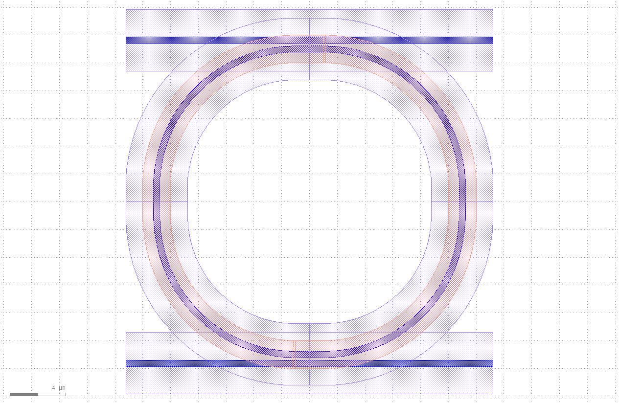
Ring resonator covered by a back-end opening layer: GDSII
Defining the virtual fabrication
A virtual fabrication is used for:
visualizing the 2D cross-sections of the structure using
visualize_2d.top-down view of the material stacks
cross_section.exporting 3D geometries, so they can be passed to a device simulator (see also physical device simulation)
More explanation on virtual fabrication, what it does and how to set it up, can be found here.
Let’s set up the virtual fabrication now:
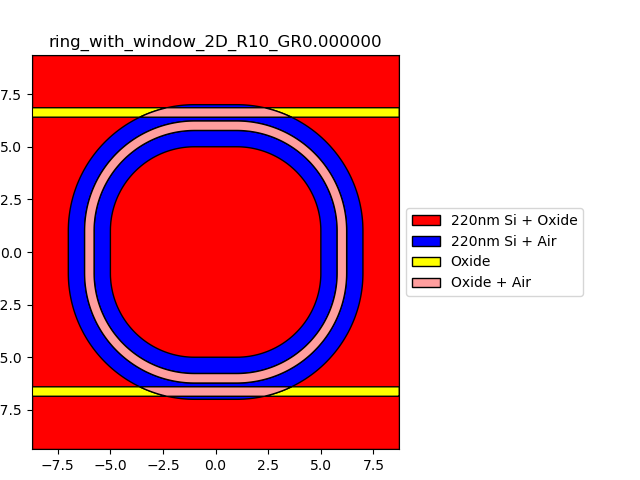
MSTACK_SOI_OX = i3.MaterialStack(
    name="Oxide",
    materials_heights=[
        (TECH.MATERIALS.SILICON_OXIDE, 1.0),
        (TECH.MATERIALS.SILICON_OXIDE, 0.22),
        (TECH.MATERIALS.SILICON_OXIDE, 1.0),
    ],
    display_style=DisplayStyle(color=color.COLOR_YELLOW),
)

MSTACK_SOI_220nm_OX = i3.MaterialStack(
    name="220nm Si + Oxide",
    materials_heights=[
        (TECH.MATERIALS.SILICON_OXIDE, 1.0),
        (TECH.MATERIALS.SILICON, 0.220),
        (TECH.MATERIALS.SILICON_OXIDE, 1.0),
    ],
    display_style=DisplayStyle(color=color.COLOR_RED),
)
MSTACK_SOI_220nm_AIR = i3.MaterialStack(
    name="220nm Si + Air",
    materials_heights=[
        (TECH.MATERIALS.SILICON_OXIDE, 1.0),
        (TECH.MATERIALS.SILICON, 0.220),
        (TECH.MATERIALS.AIR, 1.0),
    ],
    display_style=DisplayStyle(color=color.COLOR_BLUE),
)
MSTACK_OX_AIR = i3.MaterialStack(
    name="Oxide + Air",
    materials_heights=[
        (TECH.MATERIALS.SILICON_OXIDE, 1.0),
        (TECH.MATERIALS.SILICON_OXIDE, 0.220),
        (TECH.MATERIALS.AIR, 1.0),
    ],
    display_style=DisplayStyle(color=color.COLOR_ORANGE),
)

# then compose a process flow

TECH.VFABRICATION.overwrite_allowed.append("PROCESS_FLOW")
PROCESS_FLOW = i3.VFabricationProcessFlow(
    active_processes=[TECH.PROCESS.SI, TECH.PROCESS.OXIDE_OPEN],
    process_layer_map={
        TECH.PROCESS.SI: TECH.PPLAYER.SI,
        TECH.PROCESS.OXIDE_OPEN: TECH.PPLAYER.OXO.TRENCH,
    },
    process_to_material_stack_map=[  # WG, OXIDE_OPEN
        ((0, 0), MSTACK_SOI_220nm_OX),
        ((0, 1), MSTACK_SOI_220nm_AIR),
        ((1, 0), MSTACK_SOI_OX),
        ((1, 1), MSTACK_OX_AIR),
    ],
    is_lf_fabrication={
        TECH.PROCESS.SI: False,
        TECH.PROCESS.OXIDE_OPEN: False,
    },
)
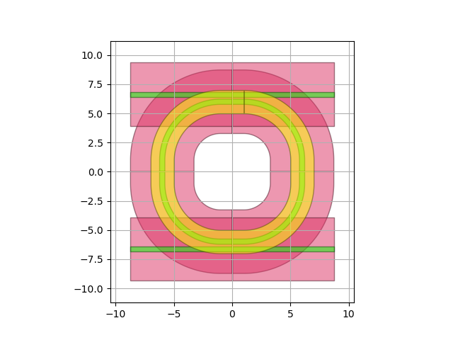
Once the PROCESS_FLOW is defined, we can call visualize_2d, and see the updated virtual fabrication:
Rlayout.visualize_2d(process_flow=PROCESS_FLOW)
<Figure size 640x480 with 1 Axes>
The default value of process_flow for visualize_2d is the PROCESS_FLOW defined in the technology.
We can persist it this way, so we can just call Rlayout.visualize_2d().
TECH.VFABRICATION.overwrite_allowed.append("PROCESS_FLOW")
TECH.VFABRICATION.PROCESS_FLOW = PROCESS_FLOW