Note
Go to the end to download the full example code
SpectrumAnalyzer: Near and Far Crosstalk
In this example, we explain how to use the i3.SpectrumAnalyzer and
the difference between the near and far crosstalk.
Let’s first create some artificial “signal” data using a Gaussian function.
import ipkiss3.all as i3
from ipkiss3.simulation.circuit.results import SMatrix1DSweep
import numpy as np


def gaussian(x, mu, sigma):
    return np.exp(-np.power(x - mu, 2.0) / (2 * np.power(sigma, 2.0)))


x = np.linspace(1.54, 1.56, 100)
yA = gaussian(x, mu=1.546, sigma=0.001) + 0.001
yB = gaussian(x, mu=1.547, sigma=0.001) + 0.001
yC = gaussian(x, mu=1.548, sigma=0.001) + 0.001
yD = gaussian(x, mu=1.553, sigma=0.001) + 0.001
From this data, we make an artificial S-matrix:
term_mode_map = {
    ("A", 0): 0,
    ("B", 0): 1,
    ("C", 0): 2,
    ("D", 0): 3,
}

smatrix = SMatrix1DSweep(
    n_ports=4,
    term_mode_map=term_mode_map,
    sweep_parameter_name="wavelength",
    sweep_parameter_values=x,
)

smatrix["A", "A", :] = yA
smatrix["A", "B", :] = smatrix["B", "A", :] = yB
smatrix["A", "C", :] = smatrix["C", "A", :] = yC
smatrix["A", "D", :] = smatrix["D", "A", :] = yD
The Spectrum Analyzer
Now, we can analyze this S-matrix using the SpectrumAnalyzer. Along with this S-matrix, we specify the input port and the output ports.
analyzer = i3.SpectrumAnalyzer(
    smatrix=smatrix,
    input_port_mode="A",
    output_port_modes=["A", "B", "C", "D"],
    dB=True,
)
Define the bands
bands = {
    "A": [(1.6, 22.5)],
    "B": [(4.5, 25.4)],
    "C": [(7.0, 17.2)],
    "D": [(29.6, 50.5)],
}
Or, you could use the cutoff_passband function to create these automatically. For instance, the bands with a maximum acceptable power loss of -30dB with respect to the peak power:
bands = analyzer.cutoff_passbands(-30)
Peaks per channel
OrderedDict([('A', array([(1.54606061, -0.00725455)],
      dtype=[('wavelength', '<f8'), ('power', '<f8')])), ('B', array([(1.54707071, -0.01300924)],
      dtype=[('wavelength', '<f8'), ('power', '<f8')])), ('C', array([(1.54808081, -0.01964927)],
      dtype=[('wavelength', '<f8'), ('power', '<f8')])), ('D', array([(1.55292929, -0.01300924)],
      dtype=[('wavelength', '<f8'), ('power', '<f8')]))])
From these peaks we know the peak wavelength and power(s) of channel “D”:
peaks_x = peaks["D"]["wavelength"]
peak_powers = peaks["D"]["power"]
peak_power = peak_powers[0]
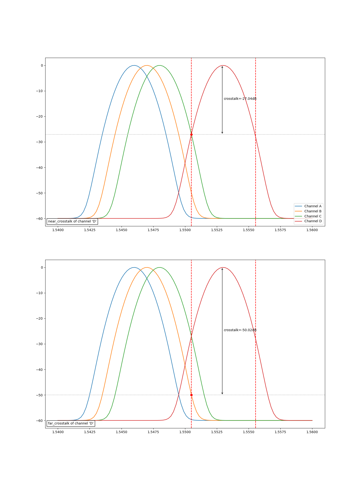
Near and Far Crosstalk
The near crosstalk calculates the maximum crosstalk with channels that are neighbouring channels.
near_crosstalk = analyzer.near_crosstalk(bands)
The far crosstalk calculates the maximum crosstalk with channels that are not neighbouring channels. For channel “D” this means the maximum crosstalk with channels “A” and “B”, because channel “C” is a neighbouring channel of “D”.
crosstalk = analyzer.crosstalk_matrix(bands)
far_crosstalk = analyzer.far_crosstalk(bands)

# The far_crosstalk of channel "D" equals the crosstalk in "D" due to "B"
# because it is bigger than the crosstalk in "D" due to "A"
assert far_crosstalk["D"] == crosstalk["D"]["B"]
assert crosstalk["D"]["B"] > crosstalk["D"]["A"]
We created a custom visualize function, specifically for this example, to show the difference between the near and
far crosstalk.
The code can be found here: visualize_crosstalk.py.
from visualize_crosstalk import visualize_crosstalk  # noqa

visualize_crosstalk(
    channel="D",
    smatrix=smatrix,
    peaks=peaks,
    near_crosstalk=near_crosstalk,
    far_crosstalk=far_crosstalk,
    bands=bands,
)