Note
Go to the end to download the full example code
A Ring Resonator based Filter based on the Vernier principle
Result
In this example, we construct a Circuit which designs a Vernier principle based filter which can act as a sensing element (e.g. biosensing). Starting from functional properties, it designs its own subcomponents. This example is based on [ClaesOE2010].
The filter consists of two ring resonators with slightly different circumference, so that a Vernier effect is obtained. When the refractive index of one of the rings (the ‘sensing’ ring) is changed, a large shift of the transmission spectrum is obtained. This shift is much larger than what can be obtained with a single ring resonator, and hence the sensitivity is considerably enhanced. This can be obtained by opening a window in the back-end oxide on top of the sensing ring, whereas the other ring resonator maintains a top cladding and can therefore not be reached by the fluid or gas which modifies the refractive index of the waveguide’s cladding. For details of the principle and operation, see [ClaesOE2010]

Vernier filter with and without refractive index difference on the sensing ring.
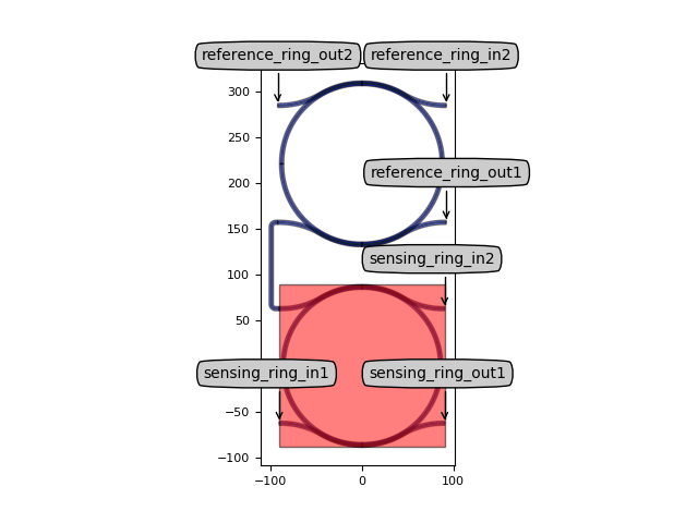
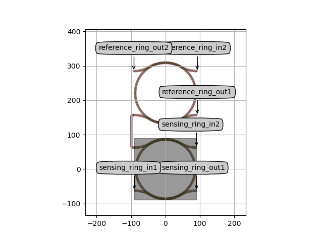
Layout of the vernier filter with two ring resonators.
Illustrates
how to define a Circuit
how to run Caphe simulations
how to use design algorithms to derive a (complex) Circuit (PCell)
Defining the Vernier Filter Circuit
We start by defining a i3.Circuit with functional parameters: the target center wavelength, the desire free spectral range of the sensing ring and the desired vernier enhancement factor.
We also specify the physical properties such as the effective and group indices, the coupler coupling coefficient, and the circumference of the rings, the trace templates to use, and two child cells (the sensing and reference ring).
class VernierFilterSensor(i3.Circuit):
    # functional parameters
    center_wavelength = i3.PositiveNumberProperty(default=1.55, doc="Center wavelength of the vernier comb.")
    target_vernier_factor = i3.PositiveNumberProperty(
        default=50.0,
        doc="Target vernier enhancement factor of the vernier filter. It will be larger than the provided value."
    )
    fsr_sensing_ring = i3.PositiveNumberProperty(
        default=0.001,
        doc="Free spectral range of the sensing ring resonator. Must be a fraction of the measurement bandwidth."
    )
    # physical properties
    coupler_coupling = i3.FractionProperty(
        default=0.5,
        doc="Coupling from the coupler to the rings. Ideally this is matched to the loss in the rings."
    )
    n_eff_sensing_ring = i3.PositiveNumberProperty(
        doc="effective index used for the measurement of the of the sensing ring. "
            "This is extracted from the model of the ring template.",
        default=2.4
    )
    n_eff_reference_ring = i3.PositiveNumberProperty(
        doc="effective used for the measurement of the of the reference ring. "
            "This is extracted from the model of the ring template.",
        default=2.4
    )
    n_g_rings = i3.PositiveNumberProperty(doc="group index of the waveguides of both rings", default=4.5)
    ring_lengths = i3.DefinitionProperty(
        restriction=i3.RestrictList(i3.RESTRICT_NONNEGATIVE),
        doc='Circumference of the ring resonators, by default calculated from functional parameters.',
    )
    # trace templates use functional parameters n_eff and n_g by default
    trace_template_sensing_ring = i3.TraceTemplateProperty(doc="Trace template used for the sensing ring.")
    trace_template_reference_ring = i3.TraceTemplateProperty(doc="Trace template used for the reference ring.")

    sensing_ring = i3.ChildCellProperty(doc="Sensing ring resonator of the vernier sensor", locked=True)
    reference_ring = i3.ChildCellProperty(doc="Reference ring resonator of the vernier sensor", locked=True)
As you can see, we reuse the logic which is already offered by Circuit,
so that we can just describe the instances and their placement, and the connections between them
to have the layout and netlist automatically generated:
class VernierFilterSensor(i3.Circuit):

    ...

    def _default_insts(self):
        return {
            "sensing_ring": self.sensing_ring,
            "reference_ring": self.reference_ring
        }


    def _default_specs(self):
        si = (self.reference_ring.get_default_view(i3.LayoutView).size_info() +
              self.sensing_ring.get_default_view(i3.LayoutView).size_info())
        d = 1.2 * si.width
        return [
            i3.Place("sensing_ring", (0.0, 0.0)),
            i3.PlaceRelative("reference_ring", "sensing_ring", (0, d)),
            i3.ConnectManhattan("sensing_ring:out2", "reference_ring:in1"),
    ]
Component synthesis by defining a design algorithm
In this example, we define the design algorithm and synthesise the components before embedding them in our Circuit. The functional design parameters were already defined above on the PCell. We also define a number of physical properties which influence the design and the behaviour of the cell:
class VernierFilterSensor(i3.Circuit):

    ...

    coupler_coupling = i3.FractionProperty(
        default=0.5,
        doc="Coupling from the coupler to the rings. Ideally this is matched to the loss in the rings.",
    )
    n_eff_sensing_ring = i3.PositiveNumberProperty(
        doc="Neff used for the measurement of the sensing ring. By default this is extracted from the caphemodel of"
        " the ring template.",
    )
    n_eff_reference_ring = i3.PositiveNumberProperty(
        doc="Neff used for the measurement of the reference ring. By default this is extracted from the caphemodel"
        " of the ring template.",
    )
    n_g_rings = i3.PositiveNumberProperty(doc="group index of the waveguides of both rings")
    ring_lengths = i3.DefinitionProperty(
        restriction=i3.RestrictList(i3.RESTRICT_NONNEGATIVE),
        doc="circumference of the ring resonators. calculated from functional parameters",
    )
The group index (n_g_rings) is used to calculate the ring resonator circumferences (ring_lengths) so that the desired fsr is obtained. The effective indices of the trace templates are used to adjust the ring resonator circumferences so that the target center wavelength is matched as closely as possible.
This design algorithm is put in a function, while the actual calculation happens when calculating the default value for ring_lengths:
...

def _calc_ring_length(center_wavelength, n_g_rings, n_eff, min_fsr, delta_order=0):
    # Gets the length of a ring so that there would be a resonance at center_wavelength at a minimum free spectral
    # range. This is done using heuristics.

    # Parameters
    # ----------
    # center_wavelength: float
    #    Center wavelength of the vernier comb.

    # n_g_rings: float
    #    Group index of the ring waveguide

    # n_eff : float
    #    Effective index of the ring waveguide

    # min_fsr : float
    #   Minimum free spectral range of the filter.

    # delta_order : float
    #   Adds delta_order to the calculated order by the filter.
    #   If delta_order is 1 the filter would have the same resonance frequency but will be a superior order.
    #   If delta_order is 1/2 the resonance wavelength would be approximately shifted by half the min_fsr.

    # Calculate the ring length that fulfills the free spectral range criterion
    ring_length_fsr = center_wavelength ** 2.0 / (n_g_rings * min_fsr)
    # Calculate the order of the ring from the length matching the FSR
    order_ring = ring_length_fsr / center_wavelength * n_eff
    # Calculate the first length that fulfills resonance and the fsr criterion
    ring_length_fsr_and_resonance = (np.floor(order_ring) + 0.5 + delta_order) * center_wavelength / n_eff
    return ring_length_fsr_and_resonance

class VernierFilterSensor(i3.Circuit):

    ...

    def _default_ring_lengths(self):
        # calculate the lengths of the rings based on the functional specs given.
        l_sensing = _calc_ring_length(
            n_eff=self.n_eff_sensing_ring,
            center_wavelength=self.center_wavelength,
            n_g_rings=self.n_g_rings,
            min_fsr=self.fsr_sensing_ring,
            delta_order=0
        )

        fsr_ref = self.fsr_sensing_ring * self.target_vernier_factor / (self.target_vernier_factor + 1)

        l_reference = _calc_ring_length(
            n_eff=self.n_eff_reference_ring,
            center_wavelength=self.center_wavelength,
            n_g_rings=self.n_g_rings,
            min_fsr=fsr_ref,
            delta_order=0
        )

        return [l_sensing, l_reference]
It is important to note that the effective index of the reference ring is used for calculating the lengths of both of the ring resonators.
The full class can be seen in vernier_filter_pcell.py
Running the design, simulation and layout
We start the main program by creating a VernierFilterSensor object and setting up the simulation environment and parameters:
import si_fab.all as pdk  # noqa

import numpy as np
import pylab as plt
from vernier_filter_pcell import VernierFilterSensor

vernier_filter = VernierFilterSensor(
    n_eff_sensing_ring=2.4,
    n_eff_reference_ring=2.4,
    n_g_rings=4.5,
)

cm1 = vernier_filter.CircuitModel()


vernier_lay = vernier_filter.Layout()
vernier_lay.visualize(annotate=True)

wavelengths = np.arange(1.53, 1.57, 2e-6)
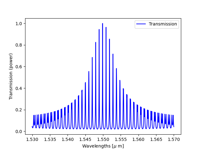
As a first step, we create the baseline design for this filter, in which the effective index of the two ring resonators is the same:
S = cm1.get_smatrix(wavelengths=wavelengths)
T1 = np.abs(S["sensing_ring_in1", "reference_ring_out2"])
# This gives the following transmission spectrum:
plt.plot(wavelengths, T1, "b", label="Transmission")
plt.xlabel(r"Wavelengths [$\mu$ m]")
plt.ylabel("Transmission (power)")
plt.legend()
<matplotlib.legend.Legend object at 0x7fdc62050d90>
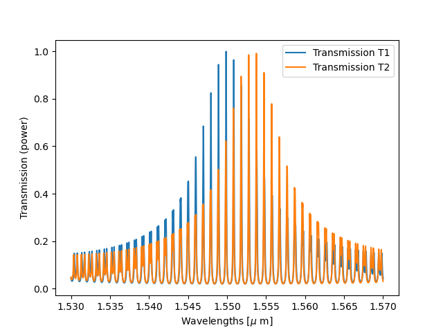
The next step is to simulate with a change on the sensing ring:
simulate with a difference in n_eff between reference and sensing ring
delta_neff = 2e-4  # effective index difference on sensing ring

vernier_filter = VernierFilterSensor(
    n_eff_sensing_ring=2.4 + delta_neff,  # We do use the vernier effect by having a change on refractive index one ring
    n_eff_reference_ring=2.4,
    n_g_rings=4.5,
)
cm2 = vernier_filter.CircuitModel()
S = cm2.get_smatrix(wavelengths=wavelengths)
T2 = np.abs(S["sensing_ring_in1", "reference_ring_out2"])
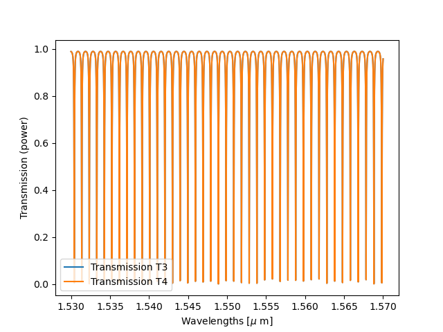
In order to compare with the influence on single ring resonators, we obtain the transmission spectra for single ring resonators by using the vernier filter’s sensing ring. In this way we don’t need to redesign the single ring to exactly match the one in the Vernier configuration.
First we design and simulate without change of effective index:
vernier_filter = VernierFilterSensor(n_eff_sensing_ring=2.4, n_eff_reference_ring=2.4, n_g_rings=4.5)
cm1 = vernier_filter.CircuitModel()
S = cm1.get_smatrix(wavelengths=wavelengths)
T3 = np.abs(S["sensing_ring_in1", "sensing_ring_out1"])
Then we extract the ring lengths from this design and create a new model, overriding the ring_lengths with the saved values. In this way, we are sure that our second simulation uses exactly the same ring resonator.
ring_lengths_v1 = vernier_filter.ring_lengths
vernier_filter = VernierFilterSensor(
    n_eff_sensing_ring=2.4 + delta_neff, n_eff_reference_ring=2.4, n_g_rings=4.5, ring_lengths=ring_lengths_v1
)
cm2 = vernier_filter.CircuitModel()
S = cm2.get_smatrix(wavelengths=wavelengths)
T4 = np.abs(S["sensing_ring_in1", "sensing_ring_out1"])
Finally, we can compare the obtained spectra (T1, T2 for the vernier filter and T3, T4 for the single ring resonators) on the graphs below:
plt.figure()
plt.plot(wavelengths, T1, label="Transmission T1")
plt.plot(wavelengths, T2, label="Transmission T2")
plt.xlabel(r"Wavelengths [$\mu$ m]")
plt.ylabel("Transmission (power)")
plt.legend()
plt.show()

plt.figure()
plt.plot(wavelengths, T3, label="Transmission T3")
plt.plot(wavelengths, T4, label="Transmission T4")
plt.xlabel(r"Wavelengths [$\mu$ m]")
plt.ylabel("Transmission (power)")
plt.legend()
plt.show()
T. Claes, W. Bogaerts, P. Bienstman, “Experimental characterization of a silicon photonic biosensor consisting of two cascaded ring resonators based on the Vernier-effect and introduction of a curve fitting method for an improved detection limit”, Optics Express 18(22), pp. 22747-22761 (2010).