camfr_mode_fields
- ipkiss3.all.device_sim.camfr_mode_fields(material_stack, wavelengths, modes=[], components=[], sample_dist=0.01)
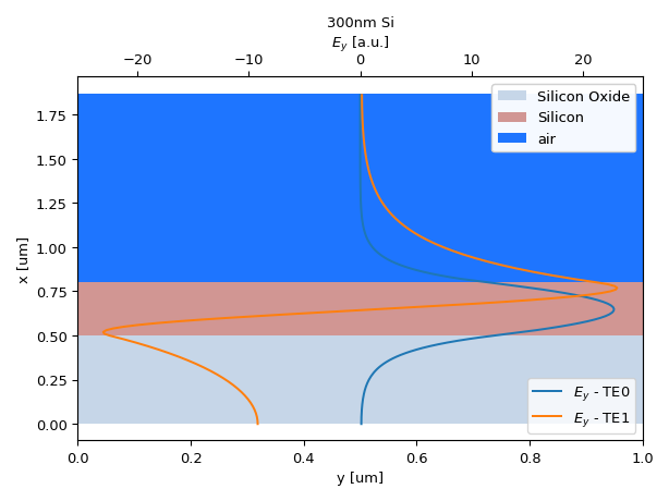
Calculates the fields for the modes for a material stack using the camfr mode solver.
This function can be useful to get insight in camfr_guided_modes, as the latter only returns the calculated neffs.
- Parameters:
- material_stack: MaterialStack object
The stack of ipkiss materials to calculate the modes for.
- wavelengths: array_like
An array of wavelengths to calculate the modes for
- modes: List[str]
A list of modenames to calculate the fields for. [‘TE0’, ‘TM1’] will select the zeroth order TE mode and the first order TM mode
- components: List[str]
A list of field components to calculate. [‘E1’, ‘E2’, ‘Ez’] will calculate all E fields
- sample_dist: float
Distance between the positions to sample the fields on.
- Returns:
- tuple
Tuple of fields and x_positions. fields is a numpy array of size (n_modes, n_wavelengths, n_components, n_x_positions) and of type np.complex128, while x_positions is an array of coordinates at which the field is sampled
Examples
import si_fab.all as pdk
from ipkiss.technology import get_technology
TECH = get_technology()
from pysics.basics.material.material_stack import MaterialStack
import ipkiss3.all as i3
import numpy as np
import matplotlib.pyplot as plt

# we define a MaterialStack
mstack = MaterialStack(
    name="300nm Si",
    materials_heights=[
        (TECH.MATERIALS.SILICON_OXIDE, 0.500),
        (TECH.MATERIALS.SILICON, 0.300),
        (TECH.MATERIALS.AIR, 1.070)
    ]
)

wavelengths = np.linspace(1.54, 1.56, 10)

# calculate the fields

fields, positions = i3.device_sim.camfr_mode_fields(
    mstack,
    wavelengths,
    modes=['TE0', 'TE1'],
    components=['E2', 'H2'],
    sample_dist=0.010
)

# we select the fields for a certain mode and
# a certain wavelength
TE0 = fields[0, 0, 0, :].real
TE1 = fields[1, 0, 0, :].real
max_fields = max(np.max(TE0), np.max(TE1))
min_fields = min(np.min(TE0), np.min(TE1))

fig = mstack.visualize(show=False, titlepad=35)
ax1 = fig.gca()
ax1.set_ylabel('x [um]')
ax1.set_xlabel('y [um]')
ax2 = ax1.twiny()

ax2.set_xlabel(r'$E_y$ [a.u.]')
ax2.plot(TE0, positions, label='$E_y$ - TE0')
ax2.plot(TE1, positions, label='$E_y$ - TE1')

# we add a legend
plt.legend(loc='lower right')
plt.tight_layout()
plt.show()