Creating compact models

Compact models

A compact model characterizes the behaviour of a component by representing it as an S-matrix and (optionally) a set of differential equations. Its use is to quickly simulate large circuits in frequency and time domain (not to do physical simulations like an FDTD or EME solver would).

Typically, a PDK already contains some predefined compact models designed for the components in the foundry’s library. However, with IPKISS, you can easily adjust these models or even create your own. In this chapter, we’ll look at the overal structure of a compact model and how you could run frequency-domain simulations for an MMI.

There are 4 steps to creating a compact model:

Create a new class, inheriting from i3.CompactModel

from ipkiss3 import all as i3
import numpy as np  # useful numerical package
import pylab as plt  # useful plotting package

# 1. We will start by looking at a compact model for a basic 1x2 MMI component. We create a new class that inherits from
# CompactModel. We then add the parameters, terms, and finally the S-matrix behaviour that describes the
# component.


class MMI1x2Model(i3.CompactModel):
    """Model for a 1x2 MMI"""

2. Define the model parameters. A parameter can be anything that influences or defines the behaviour of the component. In this case, ‘center_wavelength’ is the intended operating wavelength. The other parameters are represented by a list of polynomial coefficients used to fit the reflection and transmission from/through the MMI as a function of wavelength.

    parameters = [
        "center_wavelength",
        "reflection_in",
        "reflection_out",
        "transmission",
    ]

Specify the inputs and outputs (also referred to as ‘terms’ or ‘terminals’) of the component.

    terms = [
        i3.OpticalTerm(name="in1"),
        i3.OpticalTerm(name="out1"),
        i3.OpticalTerm(name="out2"),
    ]

4. Write down the S-matrix based on the terms and parameters. The polynomial coefficients of the reflection and transmission are evaluated at the wavelength of interest and the result is placed in the S-matrix.

    def calculate_smatrix(parameters, env, S):
        # 5. Due to symmetry in the MMI we can populate the six S-matrix terms using just three variables. If you had
        # some asymmetric data, for example measurement data, then more variables would need to be added. The
        # np.polyval() method is a numpy function that evaluates a list of polynomial coefficients
        # ordered from highest degree to the constant term. This is used to obtain an estimate for our model parameters
        # at any wavelength.

        reflection_in = np.polyval(parameters.reflection_in, env.wavelength - parameters.center_wavelength)
        reflection_out = np.polyval(parameters.reflection_out, env.wavelength - parameters.center_wavelength)
        transmission = np.polyval(parameters.transmission, env.wavelength - parameters.center_wavelength)

        S["in1", "out1"] = S["out1", "in1"] = S["in1", "out2"] = S["out2", "in1"] = transmission
        S["in1", "in1"] = reflection_in
        S["out1", "out1"] = S["out2", "out2"] = reflection_out

Later in this tutorial, we will cover how to attach this model to the MMI’s PCell. For now, we’ll use test_circuitmodel to test the response. First, the model is instantiated by filling in parameter values and, then, is simulated over a wavelength range from 1.5 to 1.6 \(\mu m\). Do not worry about where the values for transmission and ref_in come from, this will be covered later in the tutorial.

transmission = [6689915, -372855, -23043.0, 1146.79, 12.0728, -1.74281, 0.0306654, 0.694049]
ref_in = [15704086, 1274526, -92758.5, -4422.89, 185.873, 2.55599, -0.177514, 0.00621437]

wavelengths = np.linspace(1.5, 1.6, 101)  # regularly spaced array of wavelengths

S = i3.circuit_sim.test_circuitmodel(
    MMI1x2Model(
        center_wavelength=1.55,
        transmission=transmission,
        reflection_in=ref_in,
        reflection_out=np.array([0.001]),  # try changing this and re-plotting
    ),
    wavelengths=wavelengths,
)

The resulting S-matrix can be plotted using Matplotlib. The transmission and reflection values are converted to a decibel scale for easy comparison using the IPKISS function i3.signal_power_dB.

fig, ax = plt.subplots(2)
ax[0].plot(wavelengths, i3.signal_power_dB(S["out1", "in1"]), "-", linewidth=2.2, label="Transmission")
ax[1].plot(wavelengths, i3.signal_power_dB(S["out1", "out1"]), "-", c="orange", linewidth=2.2, label="Reflection_out")
ax[1].plot(wavelengths, i3.signal_power_dB(S["in1", "in1"]), "-", c="green", linewidth=2.2, label="Reflection_in")
ax[1].set_xlabel("Wavelength [$\u03BC$m]", fontsize=16)
ax[0].set_ylabel("Transmission [dB]", fontsize=16)
ax[1].set_ylabel("Reflection [dB]", fontsize=16)
ax[0].legend(fontsize=14, loc=5)
ax[1].legend(fontsize=14, loc=5)
plt.show()

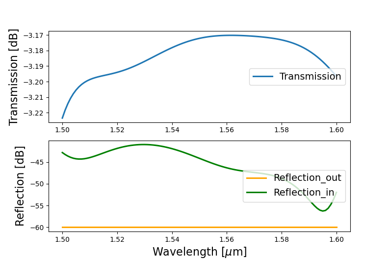
../../../_images/mmi_frequency_response.png — Frequency-domain simulation of an 1x2 MMI using a compact model

Data driven models

Using the methodology described above, it’s a small step to running the model from simulation or experimental data. As an example, we will use simulated transmission and reflection values for our MMI obtained with a third party solver. This data is then imported in Python, fitted using NumPy and passed to the compact model.

transmission = np.genfromtxt("data/transmission.csv")  # import our transmission data from a csv file using numpy
reflection_in = np.genfromtxt("data/reflection_in.csv")  # we do the same for the reflection data

# We make an arbitrary dataset for reflection_out. It is done by using "full_like" function from numpy library, that
# generates an array for reflection_out with the same shape and datatype as reflection_in.
# The value of this array are equal and are set as 0.001. Try changing this and replotting.
reflection_out = np.full_like(reflection_in, 0.001)

center_wavelength = 1.55  # we will use this to normalize our fit
wavelengths = np.linspace(1.5, 1.6, 101)  # the wavelengths that correspond to the transmission/reflection datasets

transmission_coefficients = np.polyfit(wavelengths - center_wavelength, transmission, 7)
reflection_in_coefficients = np.polyfit(wavelengths - center_wavelength, reflection_in, 7)

We use a polynomial fit to describe the data as it reduces the memory requirement and speeds up the simulation time. Instead of loading the entire dataset and interpolating for every value we need, we have described the material with only 7 numbers. As most material properties vary slowly as a function of wavelength this approximation provides very good results.

S = i3.circuit_sim.test_circuitmodel(
    MMI1x2Model(
        center_wavelength=1.55,
        transmission=transmission_coefficients,
        reflection_in=reflection_in_coefficients,
        reflection_out=reflection_out,
    ),
    wavelengths=wavelengths,
)

IPKISS also provides the method from_touchstone in case your data comes in the form of a touchstone file.

To verify the fitting and possibly adjust it, plot it together with the original data:

fig, ax = plt.subplots(2)
ax[0].plot(wavelengths, i3.signal_power_dB(S["out1", "in1"]), linestyle="-", linewidth=2, label="Transmission polyfit")
ax[0].plot(wavelengths, i3.signal_power_dB(transmission), linestyle="--", linewidth=2, label="Transmission data")
ax[1].plot(wavelengths, i3.signal_power_dB(S["in1", "in1"]), "-", linewidth=2, label="Reflection_in polyfit")
ax[1].plot(wavelengths, i3.signal_power_dB(reflection_in), "--", linewidth=2, label="Reflection_in data")
ax[1].plot(wavelengths, i3.signal_power_dB(reflection_out), "--", linewidth=2, label="Reflection_out data")

ax[1].set_xlabel("Wavelength [$\u03BC$m]", fontsize=16)
ax[1].set_ylabel("Reflection [dB]", fontsize=16)
ax[0].set_ylabel("Transmission [dB]", fontsize=16)
ax[0].legend(fontsize=14, loc=5)
ax[0].set_ylim([-7, -6])
ax[1].set_ylim([-140, -50])
ax[1].legend(fontsize=14, loc=5)
plt.show()

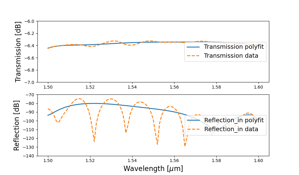
../../../_images/mmi_data_fitting.png — Frequency-domain simulation of an MMI using simulated and fitted data

In this case it would be a good idea to increase the fitting order of the reflection data to reduce the difference between the data and our model.

Component simulation

It is recommended to fit the data beforehand and store the polynomial coefficients in a file. That way, we can skip the fitting step when running a simulation and simply import the coefficients instead. This reduces the time needed to set up and run a circuit simulation.

def get_data(data_file):
    with open(data_file, "r") as f:
        results_np = json.load(f)  # the json module is included in Pyton and makes it easy to load data
    return (  # will return three objects
        results_np["center_wavelength"],
        np.array(results_np["pol_trans"]),
        np.array(results_np["pol_refl"]),
    )

At this point, we can assemble everything together and attach the model to the MMI PCell. This is done through the CircuitModel class, which acts as a container for a compact model. Similar to how the layout view describes the shape and layers of a component, the circuit model view contains information about how the component will behave in a circuit simulation.

class MMI1x2(i3.PCell):
    # 3. We will not add a layout to this class to keep this script simple, however you would add this here if you were
    # making a complete component class. Instead, we will add the CircuitModel class, and add some properties that are
    # required for our compact model.

    class CircuitModel(i3.CircuitModelView):
        center_wavelength = i3.PositiveNumberProperty(doc="Center wavelength")  # similar to layout properties
        transmission = i3.NumpyArrayProperty(doc="Polynomial coefficients for the transmission.")
        reflection_in = i3.NumpyArrayProperty(doc="Polynomial coefficients, reflection at input port.")
        reflection_out = i3.NumpyArrayProperty(doc="Polynomial coefficients, reflection at output ports.")

        def _generate_model(self):
            return MMI1x2Model(  # the model we imported from si_fab
                center_wavelength=self.center_wavelength,
                transmission=self.transmission,
                reflection_in=self.reflection_in,
                reflection_out=self.reflection_out,
            )

A simulation is started by instantiating the circuit model and calling get_smatrix.

mmi = MMI1x2()  # instantiate our class
mmi_cm = mmi.CircuitModel(  # call the CircuitModel of the class
    center_wavelength=center_wavelength,
    transmission=transmission,
    reflection_in=reflection_in,
    reflection_out=np.array([0.0]),
)

# 7. We can call the get_smatix() method for our component in the same way as we did for circuits and plot the response.
# We create a wavelength range that is valid for our fitted coefficients and plot the transmission and reflection at the
# input port.

wavelengths = np.linspace(1.5, 1.6, 101)
S = mmi_cm.get_smatrix(wavelengths=wavelengths)

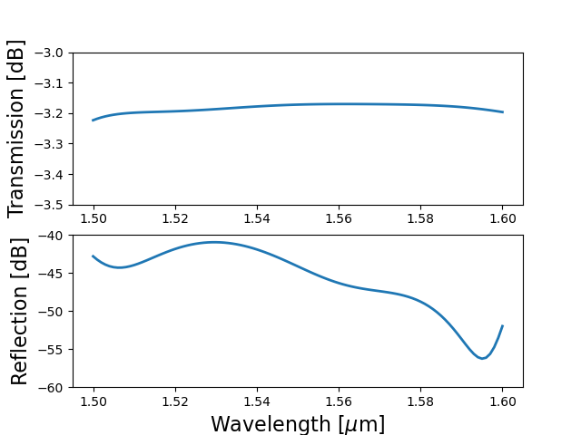
../../../_images/mmi_component_simulation.png — Frequency-domain simulation of an MMI PCell

More information

If you need more details or would like to discover what else compact models have to offer, visit our dedicated tutorial: Creating a First Circuit Simulation.
This workflow combines nicely with our links to third-party physical simulation tools, see Physical Device Simulation.
Build and optimise a passive component from scratch: Multi-mode interferometer (MMI).

Exercise

Let’s apply what we learned by creating a simple compact model for a waveguide. In getting_started/6_component_models/2_exercises/exercises.py, you will find an incomplete compact model. There are ellipses in various locations, which show you where some code needs to be added. Try to complete it, and use the solution supplied if you get stuck.