Advanced examples
Simulating a heated waveguide
Our circuit simulator ‘Caphe’ can also handle time-domain simulations. While the details are not within the scope of a getting started training, this example already gives an introduction. The first couple of steps should look familiar as the general format of the compact model is still the same.
Create a new compact model
class HeaterBroadBandPhaseErrorCompactModel(i3.CompactModel):
Add parameters.
    parameters = [
        "n_effs",
        "loss_db_per_cm",
        "wavelengths",
        "length",
        "width",
        "phase_error",
        "p_pi_sq",
        "delta_lambda",
        "v_bias_dc",
    ]
3. Add terms. We also add two electrical terms to apply a voltage difference across the waveguide.
    terms = [
        i3.OpticalTerm(name="in"),
        i3.OpticalTerm(name="out"),
        i3.ElectricalTerm(name="elec1"),
        i3.ElectricalTerm(name="elec2"),
    ]
Implement the S-matrix
    def calculate_smatrix(parameters, env, S):
        # 2. This is the usual frequency domain S-matrix response for the component. It features a phase and loss
        # calculation, hence enabling a complex expression for the transmission. There is no reflection in this model.

        neff_total = np.interp(env.wavelength, parameters.wavelengths, np.real(parameters.n_effs)) + 1j * np.interp(
            env.wavelength, parameters.wavelengths, np.imag(parameters.n_effs)
        )
        ratio = parameters.length / parameters.width
        phase_mod = np.pi * (parameters.v_bias_dc**2) / (parameters.p_pi_sq * ratio)
        beta = 2 * np.pi / env.wavelength * neff_total
        loss = 10.0 ** (-(parameters.loss_db_per_cm * 1e-4 * parameters.length) / 20.0)
        tot_phase = beta * parameters.length + parameters.phase_error * np.sqrt(parameters.length) + phase_mod
        S["in", "out"] = S["out", "in"] = loss * np.exp(1j * tot_phase)
The main difference is that two new methods are available:
calculate_signals: Captures the time dependence of the output signal on the input signal. In this case we take the length and group velocity of the waveguide into account to calculate a time delay.calculate_dydt: Includes differential equations that describe the state of the system (e.g. temperature). This part is ommitted in this example.
    def calculate_signals(parameters, env, output_signals, y, t, input_signals):
        # 3. This function defines the output_signals as function of time (t), states (y), and the input_signals.
        # The main difference is that the output signal is delayed using the length of the waveguide and the group
        # velocity of the heated waveguide.

        v_diff = abs(input_signals["elec2"] - input_signals["elec1"])
        neff_total = np.interp(env.wavelength, parameters.wavelengths, np.real(parameters.n_effs)) + 1j * np.interp(
            env.wavelength, parameters.wavelengths, np.imag(parameters.n_effs)
        )
        beta = 2 * np.pi / env.wavelength * neff_total
        ratio = parameters.length / parameters.width
        phase_mod = np.pi * (v_diff**2) / (parameters.p_pi_sq * ratio)
        tot_phase = beta * parameters.length + parameters.phase_error * np.sqrt(parameters.length) + phase_mod
        loss = 10.0 ** (-(parameters.loss_db_per_cm * 1e-4 * parameters.length) / 20.0)
        transmission = loss * np.exp(1j * tot_phase)

        neff_minus = np.interp(
            env.wavelength - parameters.delta_lambda, parameters.wavelengths, np.real(parameters.n_effs)
        )
        neff_plus = np.interp(
            env.wavelength + parameters.delta_lambda, parameters.wavelengths, np.real(parameters.n_effs)
        )
        dneff_dlambda = (neff_plus - neff_minus) / (2 * parameters.delta_lambda)
        ng = np.real(neff_total) - env.wavelength * dneff_dlambda
        t_delay = ng * parameters.length / (speed_of_light * 1e6)

        output_signals["in"] = transmission * input_signals["out", t - t_delay]
        output_signals["out"] = transmission * input_signals["in", t - t_delay]
As usual, this model can be attached to a PCell through its circuit model view.
        class CircuitModel(i3.CircuitModelView):
            # 7. We will assign parameters with a sensible default value directly (for the purposes of testing), whilst
            # other values (the wavelength range and matching effective indices) can be derived directly from the trace
            # template.

            p_pi_sq = i3.PositiveNumberProperty(default=100e-3)
            v_bias_dc = i3.NumberProperty(default=0.0)
            delta_lambda = i3.PositiveNumberProperty(default=0.001)
            loss_db_per_cm = i3.PositiveNumberProperty(default=2)

            def _generate_model(self):
                template = self.trace_template
                wavelengths = template.wavelengths
                neffs = np.array([template.get_n_eff(i3.Environment(wavelength=wl)) for wl in wavelengths])
                return HeaterBroadBandPhaseErrorCompactModel(  # return our model with completed parameters
                    length=100.0,
                    width=1.0,
                    n_effs=neffs,
                    loss_db_per_cm=self.loss_db_per_cm,
                    wavelengths=wavelengths,
                    phase_error=self.trace_template.get_phase_error(),
                    p_pi_sq=self.p_pi_sq,
                    delta_lambda=self.delta_lambda,
                    v_bias_dc=self.v_bias_dc,
                )
To run a simulation, we also need to specify some sources. We’re going to send a constant optical signal through the waveguide while linearly increasing the applied voltage.
    def ramp_function(t_rise, amplitude):
        """Returns a simple linear voltage ramping function to apply to our circuit. "t" is the current time in the
        simulation, "t_rise" is the time it takes for the voltage to ramp to its maximum, and "amplitude" is the final
        value of the applied voltage.
        """

        def f_step(t):
            if t <= t_rise:
                return amplitude * (t / t_rise)
            else:
                return amplitude

        return f_step

    dt = 1e-7  # setting up the time step variable for our simulation
    voltage_function = ramp_function(t_rise=70 * dt, amplitude=3)  # create our driving voltage function

    # 9. We will create a constant unitary optical source, and the driving voltage using the ramp function. Then we use
    # i3.ConnectComponents() to connect our component to the optical and electrical sources and an optical probe.

    optical_source = i3.FunctionExcitation(port_domain=i3.OpticalDomain, excitation_function=lambda x: 1)
    voltage_drive = i3.FunctionExcitation(port_domain=i3.ElectricalDomain, excitation_function=voltage_function)
Now, we can make a ‘testbench’ circuit that connects the sources to the waveguide, comparable to what you would do in a lab.
The simulation is started by instantiating the circuit model of the testbench circuit and running get_time_response.
    circuit = i3.ConnectComponents(
        child_cells={
            "wg": HeatedWaveguideTestCell(),  # the circuit we want to simulate
            "src_opt": optical_source,  # the optical source to be used
            "v_drive": voltage_drive,  # the drive voltage excitation
            "opt_out_probe": i3.Probe(port_domain=i3.OpticalDomain),  # our optical monitor
        },
        links=[
            ("v_drive:out", "wg:elec1"),  # connect the dc_voltage to one of the electric heaters in the circuit
            ("src_opt:out", "wg:in"),  # connect the optical source to the waveguide input
            ("wg:out", "opt_out_probe:in"),  # connect the optical probe to the waveguide output.
        ],
    )

    # 10. We can plot the results of our time domain simulation using the get_time_response() function and some common
    # Python plotting functionality. As expected, the optical power is constant as there is no loss in the model from
    # applied voltage. However, there is a constant (small) propagation loss of about 0.4% due to the length. The phase
    # changes quadratically with a linearly applied voltage for the first 70 time steps, where the ramp stops, at which
    # point a constant phase is seen for the rest of the simulation.

    result = circuit.CircuitModel().get_time_response(t0=0.0, t1=1e-5, dt=dt, center_wavelength=1.55)
The result is plotted as usual using Matplotlib:
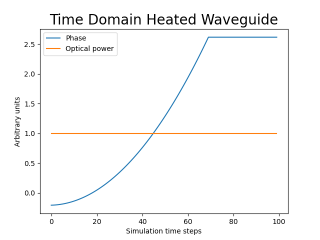
Time-domain simulation of a heated waveguide, linearly increasing the voltage across it
For more information, please visit the dedicated tutorial on circuit simulations in our documentation.