1.2. Mach-Zehnder interferometer
In this section, we are going to build a Mach-Zehnder interferometer circuit, using two Y-splitters.
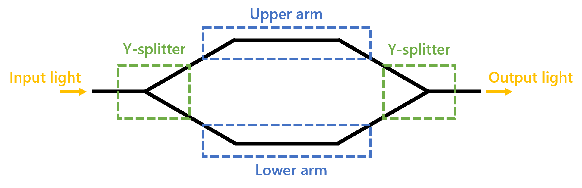
As the name suggests, a Mach-Zehnder interferometer (MZI) is an interferometric structure. In an MZI, the incoming optical wave is first split in two arms using a Y-splitter and is then recombined by a second Y-splitter. When the two beams are recombined, two different scenarios can take place:
If the two separate paths have equal optical length, the split beams are in-phase when they are recombined and constructive interference is achieved.
If the optical length of the two paths is different, the split beams will have different relative phase when they are recombined. This gives rise to destructive interference.
Therefore, depending on the relative phase difference acquired by the split beams while traveling along the two separate paths, the output light intensity can be controlled.
1.2.1. Import statements
As done before, the first step is to import all the libraries and modules we need in order to write our code.
from siepic import all as pdk
from ipkiss3 import all as i3
import pylab as plt
import numpy as np
from math import sin, pi
First, we import the Luceda PDK for SiEPIC and IPKISS. Then, we import pylab, numpy, math, which are used for plotting and for mathematical operations.
1.2.2. Instantiating the components
In order to create an MZI, we will need Y-Branch splitters and waveguides. In particular, we are going to use a straight waveguide for the bottom arm and a waveguide with a bump for the top arm. The purpose is to control the length difference between top and bottom arm (delay length) by adapting the length of the bump waveguide in the top arm.
# 1. First, we instantiate the Y-branch from the SiEPICfab PDK.
splitter = pdk.EbeamY1550()
splitter_tt = splitter.Layout().ports["opt2"].trace_template

# 2. We instantiate the waveguides we will use for the arms of the MZI.
straight_length = 200.0
delay_length = 20.0
bump_angle = get_angle(straight_length=straight_length, delay_length=delay_length, initial_angle=10.0)

wg_straight = pdk.WaveguideStraight(wg_length=straight_length, trace_template=splitter_tt)
wg_bump = pdk.WaveguideBump(x_offset=straight_length, angle=bump_angle, trace_template=splitter_tt)
First, the Y-Branch splitter is instantiated. After that, we extract the waveguide trace template from one of its port. It does not matter which port we select, as they all use the same trace template. We will need this information soon, to make sure that the waveguides use the same trace template as the ports they will be snapped to.
Afterwards, we instantiate the waveguides.
We define two parameters to control the length of the straight (bottom) waveguide (straight_length) and the delay length we want to achieve between the two arms (delay_length).
Because the waveguide bump accepts angle as parameter and not the length, we have defined a function called get_angle which allows to calculate the angle needed to achieve the desired length of the waveguide bump.
In our case, the desired length is given by straight_length + delay_length.
Check the next step if you want to learn in details how the get_angle function is defined.
Finally, we instantiate the straight waveguide with the correct length and trace template, and the bump waveguide with the desired distance between start and end point, the bump angle we calculated previously and the correct trace template.
1.2.3. (optional) The get_angle function
def get_angle(straight_length, delay_length, initial_angle):
    total_length = straight_length + delay_length
    initial_angle_rad = initial_angle * pi / 180.0

    def f(angle_rad):
        return abs(angle_rad / sin(angle_rad) - total_length / straight_length)

    from scipy.optimize import minimize

    res = minimize(
        f,
        x0=initial_angle_rad,
        bounds=((0, pi / 2),),
    ).x[0]
    angle = abs(res) * 180.0 / pi

    return angle
As explained in the previous step, the get_angle function allows to calculate the bump angle necessary to achieve a waveguide length given by straight_length + delay_length.
The meaning of ‘angle’ is described in the figure below (\(\alpha\)).
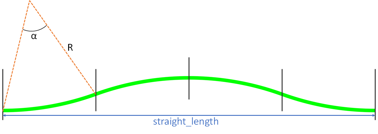
The purpose is to extract a relation between between the angle alpha and the total length of the bump waveguide based on quantities we know. The full calculation is explained in the following picture:
Our goal is therefore to solve the function \(f( \alpha )\).
Because it can’t be solved analytically, in get_angle we have chosen to solve the equation using the minimize method from the scientific Python library scipy (https://www.scipy.org/).
Finally, the function returns the result, which is the angle we will pass to WaveguideBump.
1.2.4. Building the circuit with i3.Circuit
Now that all the components we need are correctly instantiated, we can put them together in a circuit and create the MZI.
# 3. We define the cells that make up our circuit. We have 2 Y-branches, one bump waveguide and one straight waveguide.
insts = {
    "yb_1": splitter,
    "yb_2": splitter,
    "wg_up": wg_bump,
    "wg_down": wg_straight,
}

# 4. We snap the ports to each other by using `i3.Join`.
# Other placement specifications define all the transformations that apply to each instance.
specs = [
    i3.Join("yb_1:opt2", "wg_up:pin1"),
    i3.Join("wg_up:pin2", "yb_2:opt2"),
    i3.Join("yb_1:opt3", "wg_down:pin1"),
    i3.Join("wg_down:pin2", "yb_2:opt3"),
    i3.Place("yb_1:opt1", (0, 0)),
    i3.FlipH("yb_2"),
]

# 5. We define the names of the external ports that we want to access.
exposed_port_names = {
    "yb_1:opt1": "in",
    "yb_2:opt1": "out",
}

# 6. We instantiate the i3.Circuit class to create the circuit.
my_circuit = i3.Circuit(
    name="mzi",
    insts=insts,
    specs=specs,
    exposed_ports=exposed_port_names,
)
The approach used here is the same as what is used for Designing a splitter tree.
The only difference is that the components are being joined together using i3.Join instead of connectors.
In this case, we are connecting pre-instantiated components end-to-end: we are not automatically creating connectors between these components.
1.2.5. Circuit layout and simulation
We can now visualize our circuit and simulate it.
In addition to the visualization methods you learned in the previous section, here we also export the circuit to GDSII using the write_gdsii function.
Getting your design ready for tape-out is that simple!
# Layout
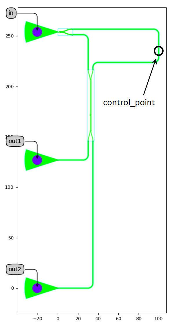
my_circuit_layout = my_circuit.Layout()
my_circuit_layout.visualize(annotate=True)
my_circuit_layout.write_gdsii("mzi.gds")
# Circuit model
my_circuit_cm = my_circuit.CircuitModel()
wavelengths = np.linspace(1.52, 1.58, 4001)
S_total = my_circuit_cm.get_smatrix(wavelengths=wavelengths)
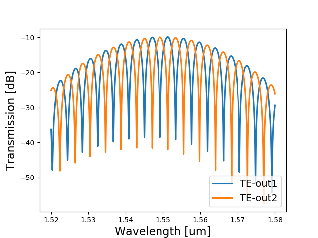
# Plotting
plt.plot(wavelengths, i3.signal_power_dB(S_total["out:0", "in:0"]), "-", linewidth=2.2, label="TE transmission")
plt.xlabel("Wavelength [um]", fontsize=16)
plt.ylabel("Transmission [dB]", fontsize=16)
plt.legend(fontsize=14, loc=4)
plt.show()
1.2.6. Test your knowledge
Now that you have all the code written down, you can try to play with it. For example, try to change the delay length and see how the circuit simulation adapts.
You may also try to implement a formula to analytically calculate the delay length from a desired value of phase shift between the two branches.