2. Rectangular PPC
In this tutorial, we show how to create a rectangular PPC in Luceda IPKISS that can be fabricated on a SiN platform:
First, we show how the MZI unit cell is designed, and find the voltages that yield the bar, cross and coupler configurations.
Then, we place a number of MZI unit cells in a 3x3 rectangular mesh and demonstrate how the optical waveguides and electrical wires can be routed to the edges of the chip.
Finally, we demonstrate how properly applying voltages to the 3x3 mesh can yield several optical functionalities for this PPC, such as tunable delays, routing and filtering.
2.1. MZI Unit Cell
The MZI unit cell consists of two 50:50 directional couplers whose ports are connected through Manhattan bends.
This allows the user to easily add a length difference between the arms (the two_arm_length_difference parameter of the unit cell).
Since the SiN platform is used, a relatively large bend radius of 50 um is used.
This value can be freely modified by adjusting the bend_radius parameter of the unit cell.
One of the arms contains the heater, or phase shifter, that allows configuring the MZI unit cell by applying a voltage bias.
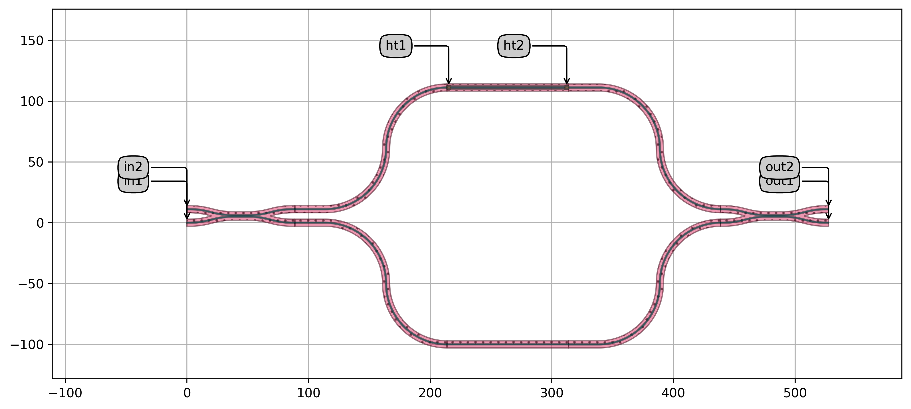
Unit cell of the SiN PPC.
The unit cell that will be used in the remainder of this tutorial is instantiated and visualized in ppc_design/example_unit_cell_layout_and_simulation.py.
One can see that the heater is placed between two straight waveguide sections of length 25 um.
This value can be freely adjusted with the wg_buffer_dx parameter of the unit cell.
The user can further decide to change the cell of the directional coupler, heater and bottom arm waveguide.
A final important attribute of the unit cell is the v_bias_dc parameter.
This parameter allows the user to run simulations, based on S-matrix calculations (that are inherently all-optical and linear), that take into account the effect of DC biases.
This will allow to calculate the S-parameters as a function of wavelength much faster and more accurately compared to time domain simulations where any delays or transients in the system need to be compensated in the post processing.
As such, to find the voltages that yield the bar, cross and coupler configuration of the MZI, we “apply” a voltage on the heater pads through v_bias_dc and sweep the voltage from 0 V to 5 V.
We then calculate the transmission between the in1 port and both the out1 and out2 ports at the center wavelength of \(1.55\,\mathrm{mu m}\) for each of the voltages from the sweep.
This is performed further on in the ppc_design/example_unit_cell_layout_and_simulation.py script, and the result is shown below:
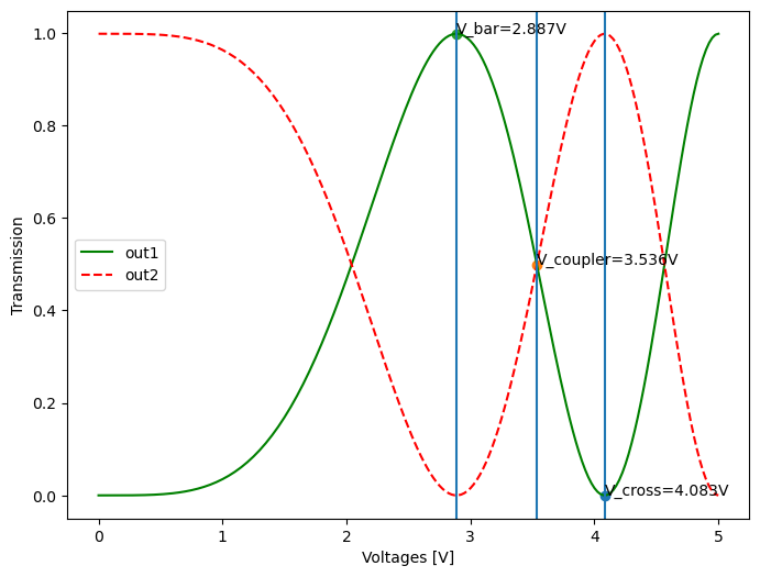
Optical power transmission of the MZI between the in1 and out1 ports (green) and in1 and out2 ports (red dashed), as a function of heater bias voltage in case the wavelength is fixed at \(\lambda=1.55\,\mathrm{\mu m}\).
From these simulation results, we can retrieve the exact values of the voltages for which we obtain the bar, cross and coupler configurations of the PPC unit cell, using the get_volts_for_min_mid_max function imported from the script located in pteam_library_si_fab/components/ppc_unit/simulation/simulate_ppc_unit_linear_voltages.py.
The values are found to be \(V_{bar}=4.083\,\mathrm{V}\), \(V_{coupler}=3.536\,\mathrm{V}\) and \(V_{cross}=2.887\,\mathrm{V}\) respectively.
This data is saved in the ppc_design/ppc_uc_voltage_biases.txt file and will be loaded when the full PPC will be simulated.
Since the coupling in the directional couplers is wavelength dependent, we check the wavelength dependence of the bar, cross and coupler configurations.
We do so over a wavelength range of 20 pm and the result is plotted below:
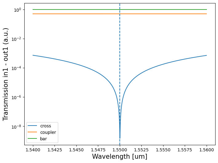
Wavelength dependence of the bar, cross and coupler configurations of the MZI switch.
One can see that the bar and coupler configurations have little wavelength dependency but that the cross state changes a lot when the wavelength is detuned from the center wavelength. In fact, due to the interpolation, the actual minimum is at a slightly different wavelength, but since the reflection is still sufficiently small at the center wavelength, we will not do further optimizations. Keeping the transmission at the cross state as low as possible is crucial in order to avoid parasitic cross talk in the programmable circuit.
2.2. Rectangular PPC Layout
It is now time to stitch together a number of the PPC unit cells in a rectangular mesh.
This is done in the script ppc_design/ppc_designs.py with the class PPCSquare.
In this class, the only parameters are:
the number of ‘squares’ in the x and y direction (\(N\) and \(M\), respectively)
the PPC unit cell (which will be placed in each side of the ‘squares’)
the side length of the ‘square’ (ideally, it is the horizontal length of the PPC unit cell, but a larger number can be given to allow more space for routing)
The unit cell that will be used is the one we discussed in the previous section.
Since we have a 3x3 mesh, we have that \(N=M=3\).
As the side length, we take 800 um.
An instance of the PPC can now be instantiated by calling PPCSquare, which is done in the example_ppc_layouts.py script.
The result (without annotated ports) is shown below.
# Instantiate the unit cell of the ppc
ppc_uc = PPCUnit(wg_buffer_dx=25.0, two_arm_length_difference=0.0, bend_radius=50.0)

# Choose the number of squares in the horizontal and vertical direction
num_v = 3
num_h = 3

# Instantiate the unrouted ppc
ppc = PPCSquare(ppc_uc=ppc_uc, num_v=num_v, num_h=num_h, side_length=800)
layout = ppc.Layout()
layout.visualize(annotate=False)
layout.write_gdsii("ppc{}{}.gds".format(num_v, num_h))
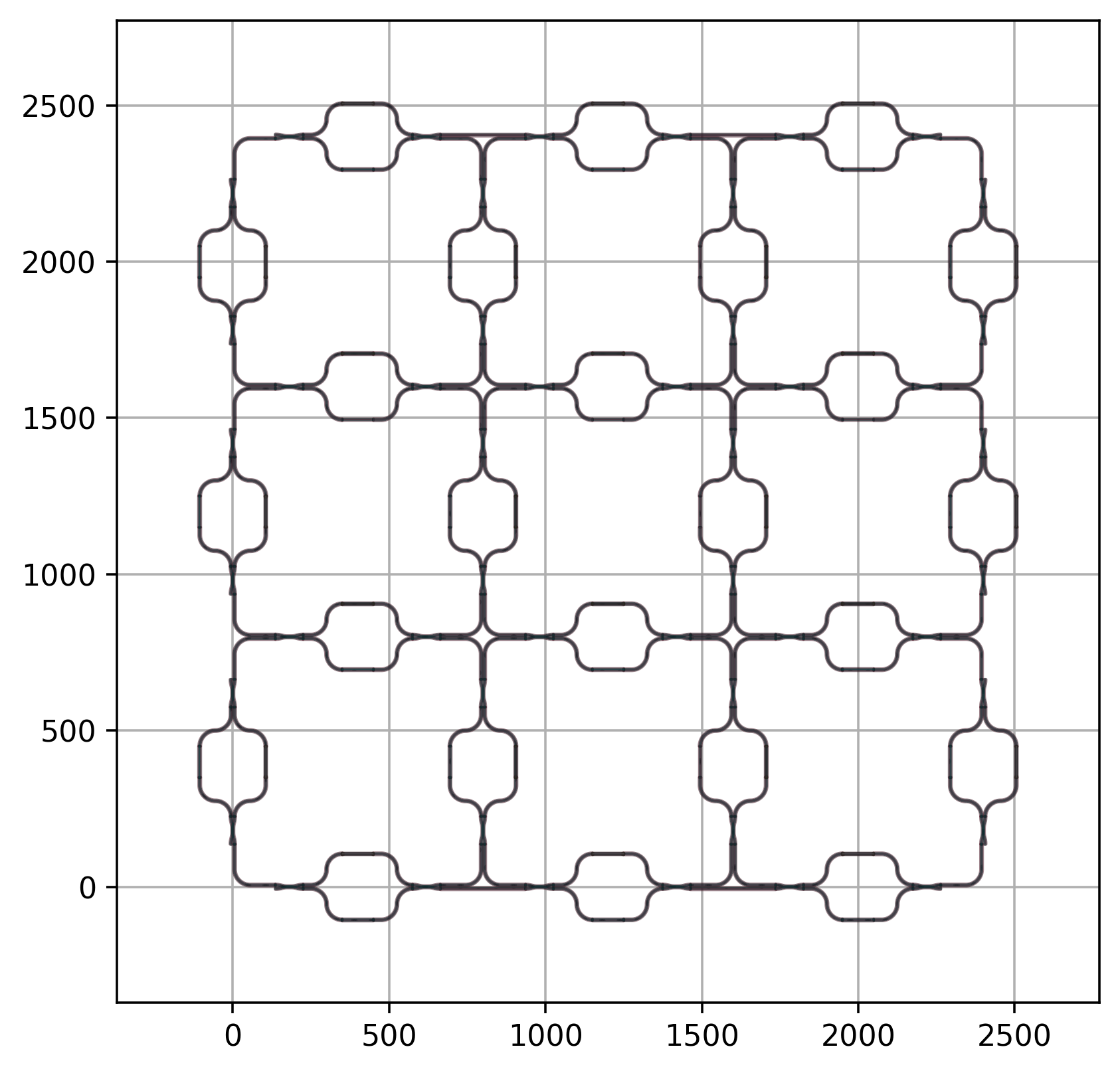
Rectangular 3x3 PPC without routing
This instance of PPCSquare can now be routed using the PPCSquareRouted class as shown further in the script.
The result is shown below.
# Instantiate the routed ppc
ppc = PPCSquareRouted(ppc=ppc, h_offset=110, v_offset=350, ec_deviation=1500, bp_deviation=1000)
layout = ppc.Layout()
layout.visualize(annotate=False)
layout.write_gdsii("ppc{}{}_routed.gds".format(num_v, num_h))
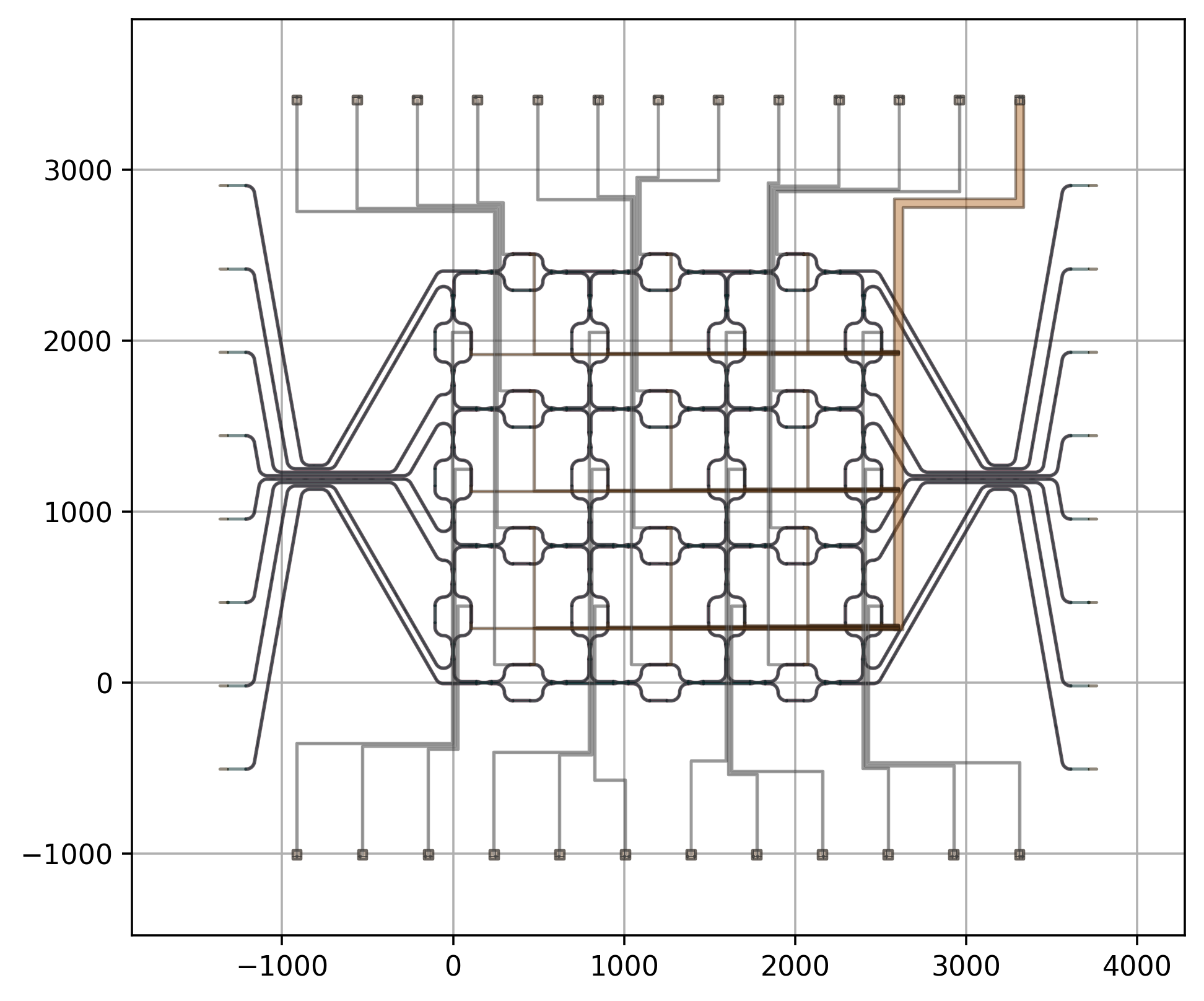
Rectangular 3x3 PPC whose optical and electrical ports are routed towards the edge couplers and metal bondpads respectively
As can be seen from the figure, the 3x3 PPC consists of 24 unit cells (or unique “square” sides):
12 horizontally placed unit cells: 4 rows, each containing 3 unit cells
12 vertically placed unit cells: 4 columns, each containing 3 unit cells
Since the optical input and output ports of the PPC are only present on the left and right side of the PPC, they are respectively routed to the edge couplers on the left and right side of the chip as well. To route the electrical wires to the heaters, the bondpads (electrical I/Os) are placed at the top and bottom of the chip. The electrical input port of the heaters in the horizontally placed unit cells are routed to the top bondpads, while for the heaters in the vertically placed unit cells, the electric wires are routed to the bottom bondpads. The ground ports of all the heaters are routed to a single wide metal track on the right, which is connected to the bondpad in the top right corner of the chip. Note that as more ground ports are connected, the width of their common ground wire becomes increasingly larger in order to lower the electric resistance and the resulting Ohmic heating. This is done by making sure the ground wires slightly overlap with each other and are routed along the same path towards the single wide metal track that is connected to the common ground bondpad.
# Get the complete schematic visualized in IPKISS CANVAS
settings = i3.NetlistExtractionSettings(
    electrical=True,
    connected_layers=[
        (i3.TECH.PPLAYER.V12, i3.TECH.PPLAYER.M1),
        (i3.TECH.PPLAYER.V12, i3.TECH.PPLAYER.M2),
    ],
)

layout.to_canvas(project_name="PPCSquareRouted", netlist_extraction_settings=settings)
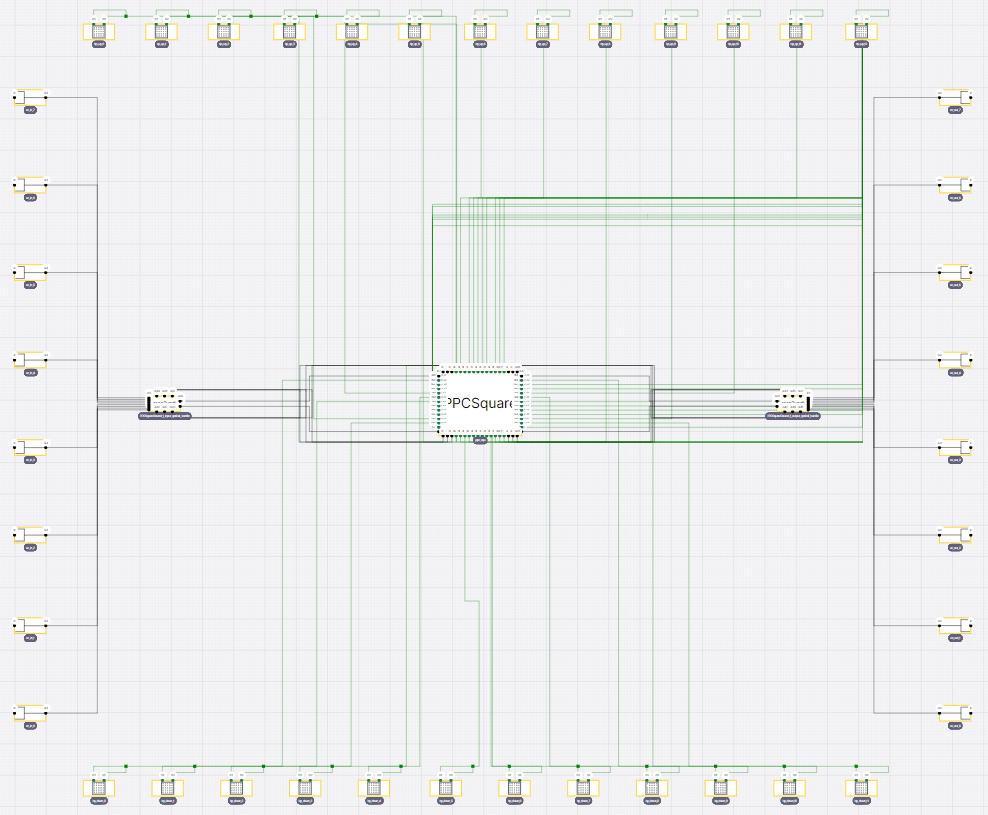
Rectangular routed 3x3 PPC schematic in Canvas
Now let’s have a look at the schematic of routed ppc in IPKISS CANVAS.
For the multi-layer connections shown in routed ppc, we need to manually specify which layers are connected
by using i3.NetlistExtractionSettings and
setting the connected_layers argument. Then we can get the complete schematic visualized
in IPKISS Canvas by to_canvas.The project (PPCSquareRouted.icproject)
will be generated in the same folder.
2.3. Reconfiguring the PPC
We will now realize different functionalities with this 3x3 PPC by simply changing the voltages on the switches that make up the PPC.
These are all implemented in the example_ppc_simulation.py script and running this script will show all three examples.
2.3.1. Tunable delay
The first functionality we are looking at is a tunable delay between the in0 and out0 optical ports.
The delay is tuned by routing the light over a different amount of unit cell sides.
In the simulation example, we look at light being routed over 3, 5 and 9 unit cell sides, which is achieved by configuring the MZI switches as shown below:
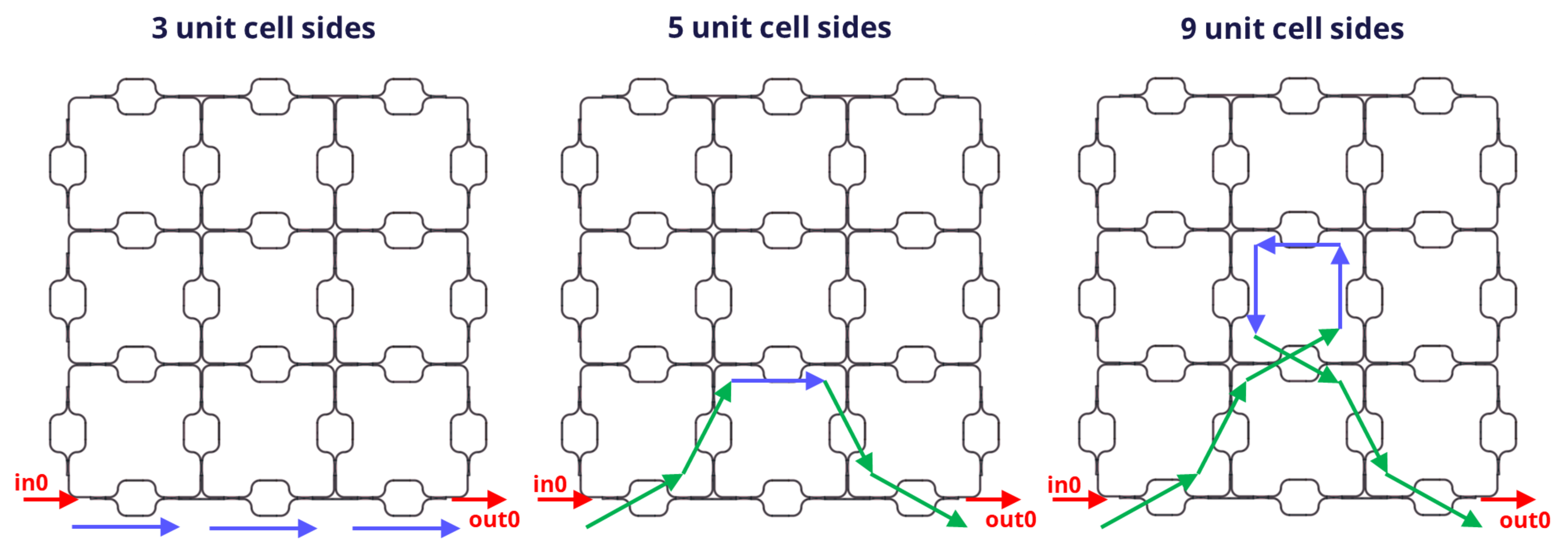
Configurations of the PPC to attain different delays. Blue and green arrows indicate the MZI is configured as bar and cross respectively.
The simulation test bench simulate_ppc is loaded from the ppc_design/ppc_simulation_test_benches.py file.
Important parameters of this function are the PPC that needs to be simulated, the voltage matrices (the voltages applied to the different MZI switches), time domain settings and center wavelength.
This test bench will launch a Gaussian pulse in the in0 port of the PPC and look at the optical power at the out0 port.
The voltage matrices to configure the PPC are given by tunable_delay_voltages_hor and tunable_delay_voltages_ver and passed on to simulate_ppc.
The simulation result is given below.
# Tunable delay line
# Show the delay in case the light routed over 3, 5 or 9 unit cell sides

print("Demonstrating tunable delay line functionality")

delay_voltages_hor = [
    [[v_bar, v_bar, v_bar], [v_bar, v_bar, v_bar], [v_bar, v_bar, v_bar], [v_bar, v_bar, v_bar]],  # 3 unit cell sides
    [  # 5 unit cell sides
        [v_cross, v_bar, v_cross],
        [v_bar, v_bar, v_bar],
        [v_bar, v_bar, v_bar],
        [v_bar, v_bar, v_bar],
    ],
    [  # 9 unit cell sides
        [v_cross, v_bar, v_cross],
        [v_bar, v_cross, v_bar],
        [v_bar, v_bar, v_bar],
        [v_bar, v_bar, v_bar],
    ],
]
delay_voltages_ver = [
    [[v_bar, v_bar, v_bar, v_bar], [v_bar, v_bar, v_bar, v_bar], [v_bar, v_bar, v_bar, v_bar]],  # 3 unit cell sides
    [[v_bar, v_cross, v_cross, v_bar], [v_bar, v_bar, v_bar, v_bar], [v_bar, v_bar, v_bar, v_bar]],  # 5 unit cell sides
    [[v_bar, v_cross, v_cross, v_bar], [v_bar, v_bar, v_bar, v_bar], [v_bar, v_bar, v_bar, v_bar]],  # 9 unit cell sides
]
plot_labels = ["3 unit cell sides", "5 unit cell sides", "9 unit cell sides"]

fig = plt.figure(figsize=(9, 6))
for v_hor, v_ver, label in zip(delay_voltages_hor, delay_voltages_ver, plot_labels):
    result = simulate_ppc(ppc_cell=ppc, voltages_hor=v_hor, voltages_ver=v_ver, center_wavelength=1.55)
    if label == plot_labels[0]:
        plt.plot(result.timesteps * 1e9, i3.signal_power(result["optical_in"]), "r--", label="in0")
    plt.plot(result.timesteps * 1e9, i3.signal_power(result["out0"]), "-", label="out0 {}".format(label))

plt.xlabel("Time (ns)", fontsize=15)
plt.ylabel("Optical output power", fontsize=15)
plt.title("Tunable delay functionality", fontsize=20)
plt.legend()
plt.show()
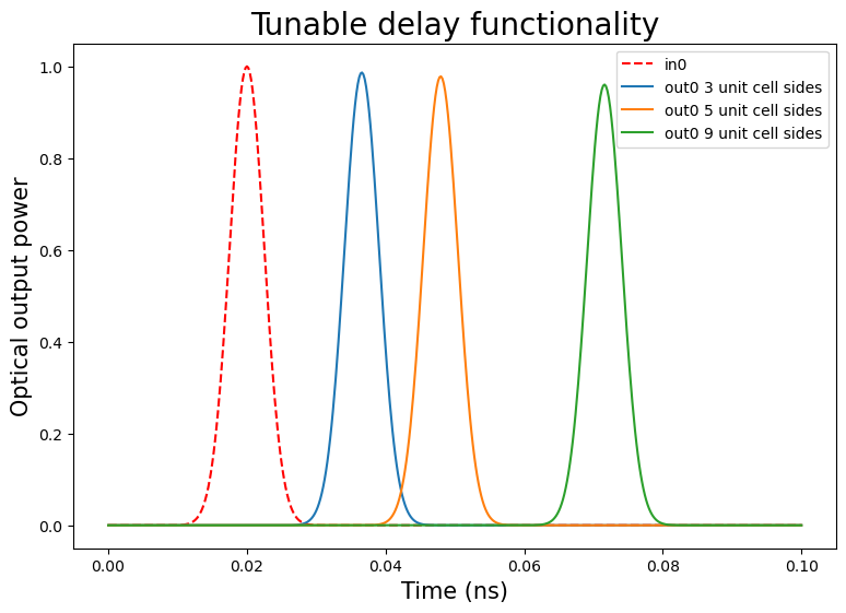
Demonstration of different delays being achieved on the 3x3 PPC.
One can clearly see that the pulse arrives at different times due to the fact the light is routed over different path lengths between the in0 and out0 optical ports.
2.3.2. Tunable routing network
The second functionality we are looking at is a tunable routing network between the in and out optical ports.
In the simulation example, we look at 2 different routing networks.
These are schematically visualised in the figure below, together with how the MZI switches are configured:
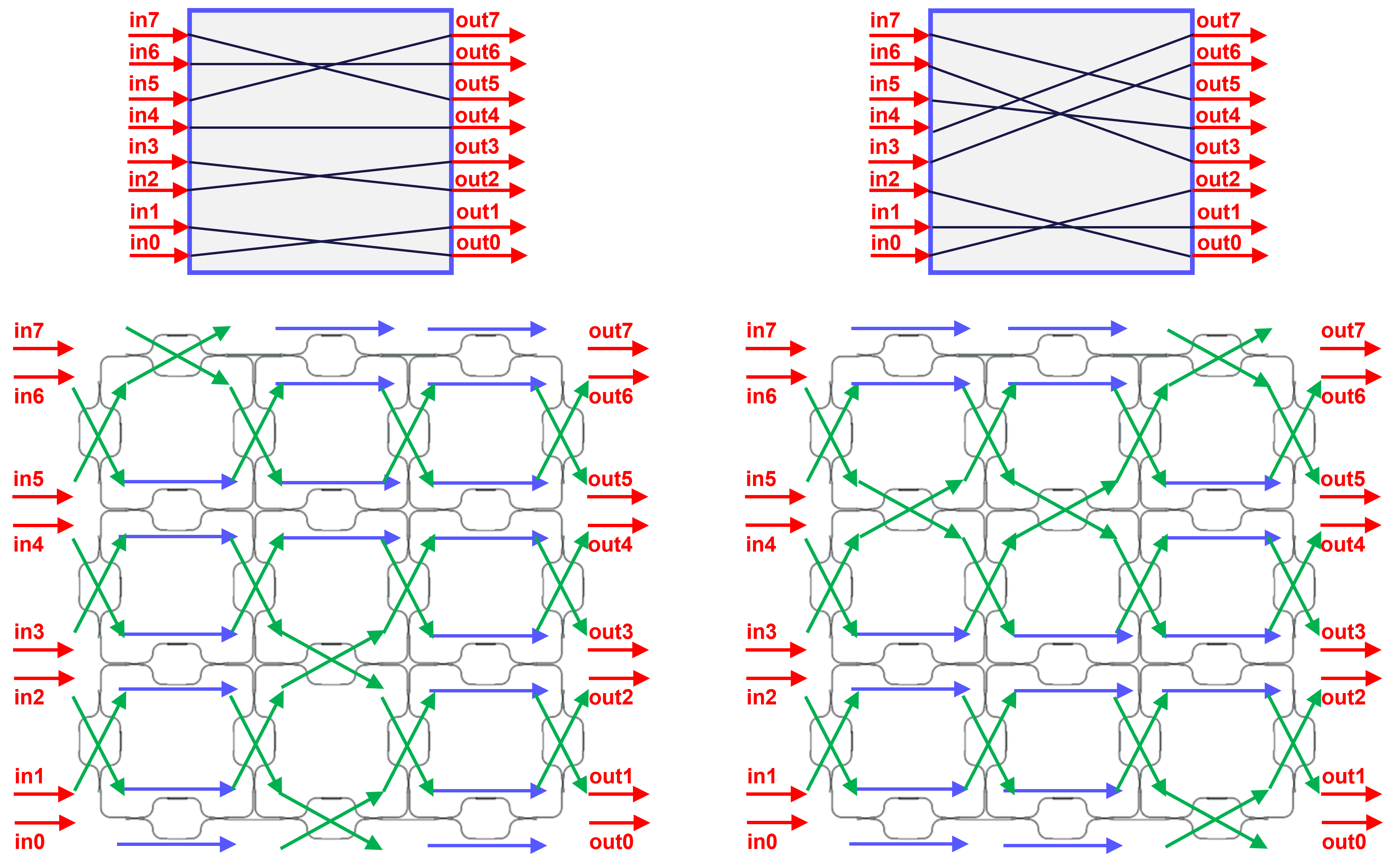
Configurations of the PPC to attain different routing networks. Blue and green arrows indicate the MZI is configured as bar and cross respectively.
The simulation testbench simulate_ppc_multi_inputs for this demonstration is loaded from the ppc_design/ppc_simulation_test_benches.py file.
Important parameters of this function are the PPC that needs to be simulated, the voltage matrices (the voltages applied to the different MZI switches), time domain settings, center wavelength and properties of the rectangular pulses.
This test bench will launch rectangular pulses in the in ports of the PPC (with a certain delay between them to improve the visualisation) and look at the optical power at the out ports.
The voltage matrices to configure the PPC are given by routing_voltages_hor and routing_voltages_ver and passed on to simulate_ppc.
The simulation result is given below:
# Tunable routing circuit
# The input optical ports are routed to the user defined output optical ports

print("Demonstrating tuneable routing functionality")

routing_voltages_hor = [
    [  # routing network 1
        [v_bar, v_cross, v_bar],
        [v_bar, v_cross, v_bar],
        [v_bar, v_bar, v_bar],
        [v_cross, v_bar, v_bar],
    ],
    [  # routing network 2
        [v_bar, v_bar, v_cross],
        [v_bar, v_bar, v_bar],
        [v_cross, v_cross, v_bar],
        [v_bar, v_bar, v_cross],
    ],
]
# the voltages on the vertical MZI switches remain unchanged in both network configurations
routing_voltages_ver = [
    [v_cross, v_cross, v_cross, v_cross],
    [v_cross, v_cross, v_cross, v_cross],
    [v_cross, v_cross, v_cross, v_cross],
]

color_values = ["blue", "green", "red", "cyan", "purple", "orange", "brown", "gray"]

fig = plt.figure(figsize=(9, 9))
for v_hor in routing_voltages_hor:
    result = simulate_ppc_multi_inputs(
        ppc_cell=ppc, voltages_hor=v_hor, voltages_ver=routing_voltages_ver, center_wavelength=1.55
    )
    if v_hor == routing_voltages_hor[0]:
        plt.subplot(211)
        plt.title("Tunable routing functionality", fontsize=20)
    else:
        plt.subplot(212)
    for m in range((ppc.num_v + 1) * 2):
        plt.plot(
            result.timesteps * 1e9,
            i3.signal_power(result["optical_in_{}".format(m)]),
            color=color_values[m],
            label="in{}".format(m),
            linewidth=2,
        )
        plt.plot(
            result.timesteps * 1e9,
            i3.signal_power(result["out{}".format(m)]),
            color=color_values[m],
            label="out{}".format(m),
            linewidth=2,
            linestyle="dashed",
        )
    plt.xlabel("Time (ns)", fontsize=15)
    plt.ylabel("Optical output power", fontsize=15)
    plt.legend()
    plt.show()
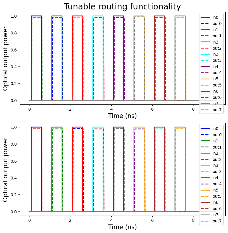
Demonstration of the two different routing networks being achieved on the 3x3 PPC.
One can clearly see that the pulses arrives at different output ports to the fact the light is routed over different paths between the in and out optical ports.
2.3.3. Tunable ring resonator
The third functionality we are looking at is a tunable ring resonator between the in0 and out0 optical ports.
In the simulation example, we look at 2 ring resonators with different ring length, which is done by rerouting the light over a different amount of unit cells.
The way the MZI switches are configured is shown below:
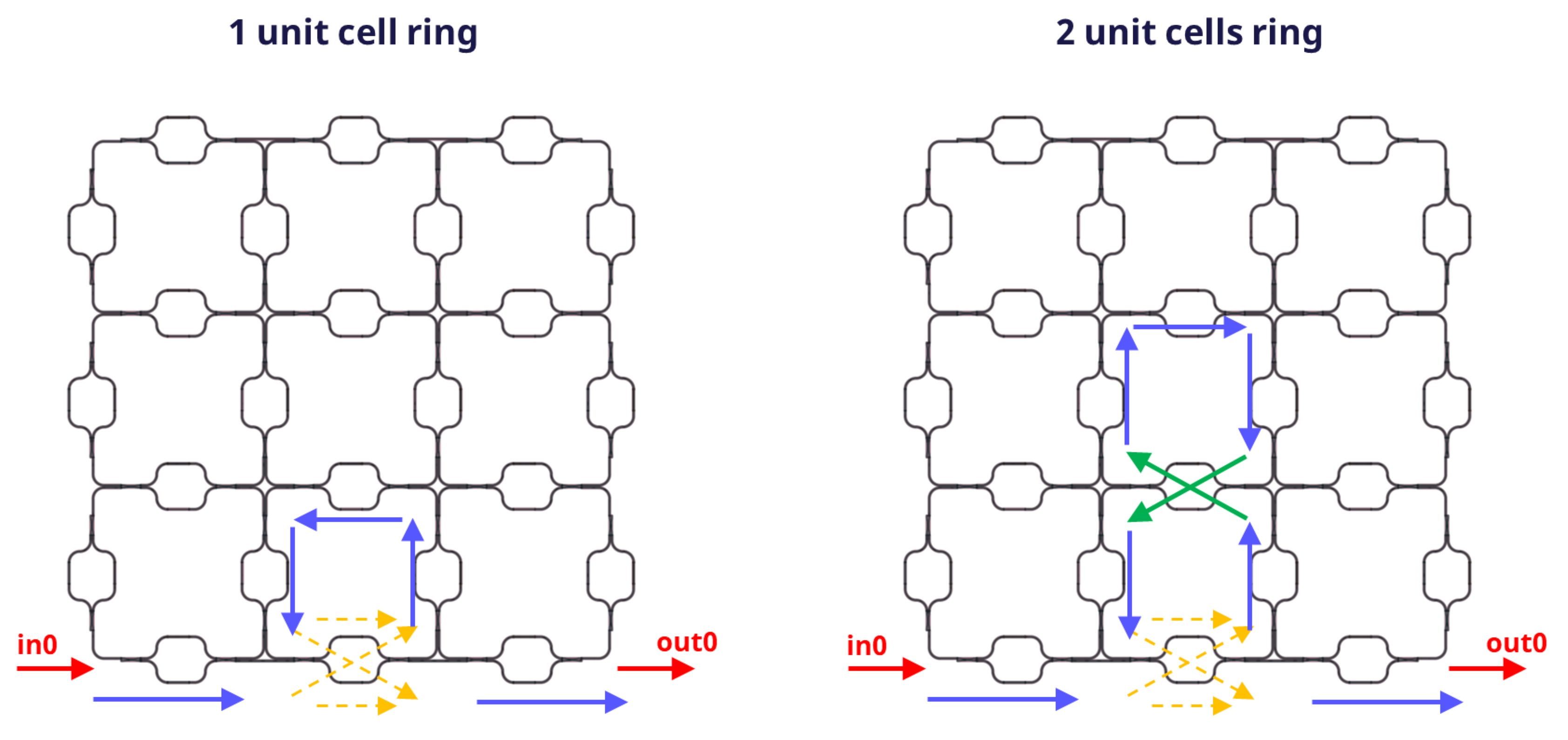
Configurations of the PPC to attain ring resonators with different length. Blue, orange and green arrows indicate the MZI is configured as bar, coupler, and cross respectively.
Since for the ring resonators we are mostly interested in its transmission spectra as a function of wavelength in order to analyze the resonances, we will perform S-matrix calculations on the PPC.
The voltages on the MZI switches are set by simply setting the v_bias_dc_hor and v_bias_dc_ver attributes of the PPC with the voltage matrices.
These are saved in the routing_voltages_hor and routing_voltages_ver variables.
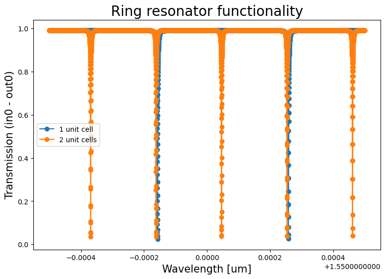
The transmission between the in0 and out0 optical ports at 1001 wavelengths over a 1 pm range around 1.55 um are now calculated for the different ring length configurations.
The simulation results are given below:
# Ring resonator simulations
# Show the ring resonator response in the wavelength domain (using S-matrix calculations by changing the attributes
# "v_bias_dc_hor" and "v_bias_dc_ver" accordingly) in case the ring consists of 1 or 2 unit cells.

print("Demonstrating ring resonator functionality")

ring_resonator_voltages_hor = [
    [  # 1 unit cell
        [v_bar, v_coupler, v_bar],
        [v_bar, v_bar, v_bar],
        [v_bar, v_bar, v_bar],
        [v_bar, v_bar, v_bar],
    ],
    [  # 2 unit cells
        [v_bar, v_coupler, v_bar],
        [v_bar, v_cross, v_bar],
        [v_bar, v_bar, v_bar],
        [v_bar, v_bar, v_bar],
    ],
]
# the voltages on the vertical MZI switches remain unchanged in both ring resonator configurations
ring_resonator_voltages_ver = [
    [v_bar, v_bar, v_bar, v_bar],
    [v_bar, v_bar, v_bar, v_bar],
    [v_bar, v_bar, v_bar, v_bar],
]
plot_labels = ["1 unit cell", "2 unit cells"]

wavelengths = np.linspace(1.5495, 1.5505, 1001)
fig = plt.figure(figsize=(9, 6))
for v_hor, label in zip(ring_resonator_voltages_hor, plot_labels):
    ppc.v_bias_dc_hor = v_hor
    ppc.v_bias_dc_ver = ring_resonator_voltages_ver
    ppc_cm = ppc.CircuitModel()
    S = ppc_cm.get_smatrix(wavelengths=wavelengths)
    transmission = np.abs(S["out0", "in0"]) ** 2
    plt.plot(wavelengths, transmission, "o-", label=label)
plt.xlabel("Wavelength [um]", fontsize=15)
plt.ylabel("Transmission (in0 - out0)", fontsize=15)
plt.title("Tunable ring resonator functionality", fontsize=20)
plt.legend()
plt.show()
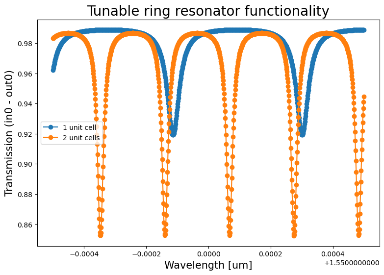
Demonstration of the two different ring resonators being achieved on the 3x3 PPC.
One can clearly see that the resonances (corresponding to the dips in the transmission spectra) are closer together in the ring with the longer ring length than with the shorter ring length. This is to be expected, because the free spectral range (FSR) or the spectral distance between the resonances of a ring resonator is inversely proportional to the ring length.
2.3.4. Exercise - Ring resonator
In the ring resonator example, one of the MZI switches is configured as coupler.
The voltage on this MZI switch is such that the power on one input port is split 50:50 over the output ports of the MZI switch.
However, most ring resonators are designed to operate at critical coupling, where the power at the resonance dips drops to or close to 0 mW.
This is clearly not the case for the ring resonators discussed in the previous subsection.
So as an exercise, we ask you to find the voltages v_coupler for which critical coupling is achieved in both rings.
The solution can be found by running the script ppc_design/ppc_ring_resonator_find_critical_coupling_voltages.py, where the optimal coupler voltages are calculated and saved in the ppc_ring_resonator_v_coupler_critical_coupling.txt text file (running this script might take a bit of time).
These values are then loaded in example_ppc_ring_resonators_at_critical_coupling_simulation.py in order to calculate the spectra of the rings operating at critical coupling.
The spectra are shown below:
Spectra of the aforementioned ring resonators operating at critical coupling.