Advanced examples

Parametric splitter tree

We’ll reuse the parametric splitter tree that was designed in the previous tutorial on circuit layout. As layout and simulation are tightly linked because of how we implemented it, it’s now possible to run a circuit simulation of a splitter tree with any number of levels. Everything changes automatically by simply changing one parameter, n_levels, of our PCell:

from si_fab import all as pdk  # noqa: F401
import numpy as np
from circuits_to_simulate import ParametricSplitterTree  # import the circuit to simulate

splitter_tree = ParametricSplitterTree(n_levels=4)
splitter_tree_lv = splitter_tree.Layout()
splitter_tree_model = splitter_tree.CircuitModel()
# splitter_tree_lv.visualize(annotate=True)  # toggle this with Ctrl+/ to visualize the circuit

wavelengths = np.linspace(1.5, 1.6, 501)
S_total = splitter_tree_model.get_smatrix(wavelengths=wavelengths)

To visualize the final S-matrix, we loop over all the output ports to construct the term_pairs list and visualize the S-matrix:

term_pairs = []
for port in range(2**splitter_tree.n_levels):
    term_pairs.append(("in", f"out{port+1}"))

S_total.visualize(term_pairs=term_pairs, scale="dB", ylabel="Transmission [dB]", figsize=(9, 5))

# 3. As all the splitters are identical, we see the response in each port is also identical, but as you
# increase the number of levels, the insertion loss increases linearly with each new level.

S_total.visualize(term_pairs=[("in", "in")], scale="dB", ylabel="Reflection [dB]", figsize=(9, 5))

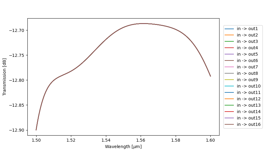
Frequency-domain simulation of a four-level splitter tree: transmission

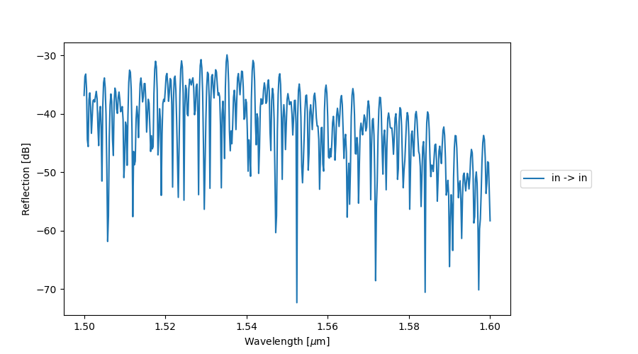
Frequency-domain simulation of a four-level splitter tree: reflection

Simulation analysis

IPKISS also provides tools to analyze spectrums and extract various characteristics like the free spectral range (FSR), insertion loss, cross talk, etc. To demonstrate this, we’ll extend the code from the tutorial where an MMI was simulated for a few path length differences. Not much has to be changed, except that the S-matrices are now passed to i3.SpectrumAnalyzer:

wavelength_range = np.linspace(1.54, 1.56, 1001)  # our wavelength range for the simulation
path_differences = np.linspace(100, 300, 9)  # range from 100 to 300 um, in steps of 25 um

results = {}

for path_difference in path_differences:
    # call the CircuitModel() method on each new MZI
    mzi_model = MZI(arm_separation=300.0, path_difference=path_difference).CircuitModel()
    s_matrix = mzi_model.get_smatrix(wavelength_range)  # extract the s-matrix
    analyzer = i3.SpectrumAnalyzer(  # using the spectrum analyser on our s-matrix between the input and output ports
        smatrix=s_matrix, input_port_mode="in", output_port_modes=["out"], dB=True, bandpass=True
    )

Next, the spectrum analyzer calculates the insertion loss, extinction ratio and FSR and the results are saved to a dictionary:

    insertion_loss = analyzer.min_insertion_losses()["out"]
    extinction_ratio = analyzer.max_insertion_losses()["out"] - analyzer.min_insertion_losses()["out"]
    fsr = np.mean(analyzer.fsr()["out"])

    results[path_difference] = [insertion_loss, extinction_ratio, fsr * 1000]  # store in the results dictionary

Finally, we can plot the characteristics as a function of the path length difference:

fig, axs = plt.subplots(nrows=3, sharex="all")  # create our plot and share the x-axis between the three subplots
plt.suptitle("MZI analysis", size=20)

for path in path_differences:
    axs[0].scatter(int(path), results[path][0], marker="x", color="b", s=50)
    axs[1].scatter(int(path), results[path][1], marker="x", color="b", s=50)
    axs[2].scatter(int(path), results[path][2], marker="x", color="b", s=50)

axs[0].set_ylabel("Insertion loss [dB]", fontsize=15)  # add a y-label to each subplot that is the same
axs[1].set_ylabel("Extinction ratio [dB]", fontsize=15)  # add a y-label to each subplot that is the same
axs[2].set_ylabel("FSR [nm]", fontsize=15)  # add a y-label to each subplot that is the same
axs[2].set_xlabel("Path difference [\u03BCm]", fontsize=15)
plt.show()

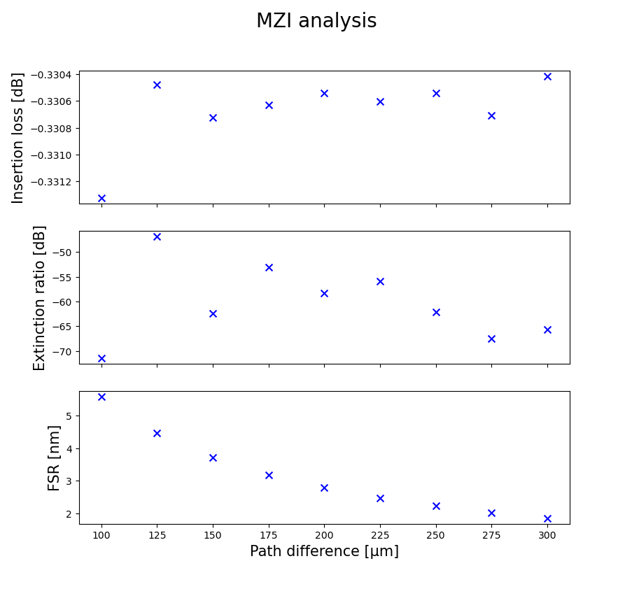
Performance analysis of an MZI using i3.SpectrumAnalyzer