Ansys Lumerical FDTD
When you set up an electromagnetic simulation using Ansys Lumerical FDTD from within IPKISS, you go through the following steps:
Define the geometry that represents your component.
Specify the simulation job, consisting of the geometry, the expected outputs and simulation settings
Inspect the exported geometry
Retrieve the simulation results
1. Define the geometry
We’ve already covered step 1 by creating a SimulationGeometry for an MMI. However we will adjust the geometry a bit by growing the waveguides slightly:
sim_geom = i3.device_sim.SimulationGeometry(
    layout=MMI_lo,
    waveguide_growth=0.1,
)
This makes sure the ports don’t fall at the edge of the simulation region. The next step is to create an object that will handle the simulations.
2. Define the simulation
To create a simulation using the geometry we’ve just defined, we’ll instantiate an
i3.device_sim.LumericalFDTDSimulation object:
simulation = i3.device_sim.LumericalFDTDSimulation(
    geometry=sim_geom,
    outputs=[
        i3.device_sim.SMatrixOutput(
            name='smatrix',
            wavelength_range=(1.5, 1.6, 100),
            symmetries=[('out1', 'out2')]
        )
    ],
    setup_macros=[
        i3.device_sim.lumerical_macros.fdtd_mesh_accuracy(2),
        i3.device_sim.lumerical_macros.fdtd_profile_xy('out1')
    ]
)
Apart from the simulation geometry we also have to specify an output.
By using SMatrixOutput, the simulator will perform
an S-parameter sweep and return an SMatrix (i3.circuit_sim.Smatrix1DSweep).
Note that we can use the symmetry of the MMI to speed up the calculation. This is done by setting
the symmetries argument of SMatrixOutput.
We have also added two macros:
fdtd_mesh_accuracyallows to control the meshing accuracy of the component in Lumerical FDTD. A mesh accuracy of 1 means a coarse grid will be used and thus the computation should go more quickly. For accurate results it is recommended to use a mesh accuracy of at least 2.fdtd_profile_xylets us place a monitor on a port and visualize the results (like the electric field) after the simulation is done.
Now everything is set up to start Ansys Lumerical FDTD and do our first simulation.
3. Inspect the simulation job
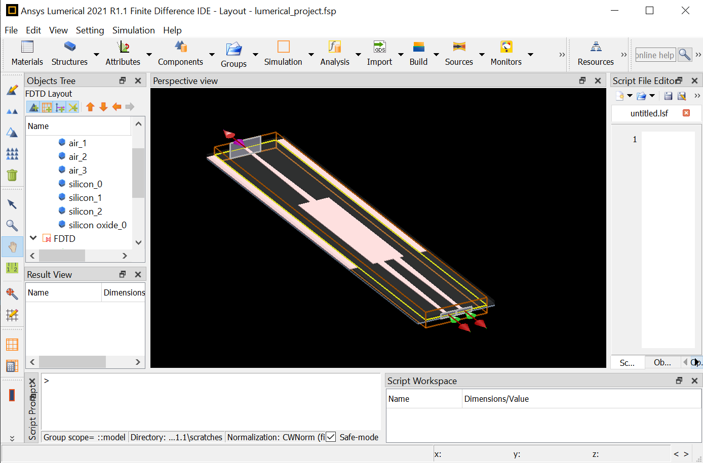
To see what it looks like, you can use the inspect method:
simulation.inspect()
The FDTD Solutions graphical user interface will open twice. First, the GUI will be opened to build up the geometry and settings in an automated way. Then, the GUI will close and re-open for inspection. This is for technical implementation reasons.
After execution, the FDTD Solutions GUI will open:
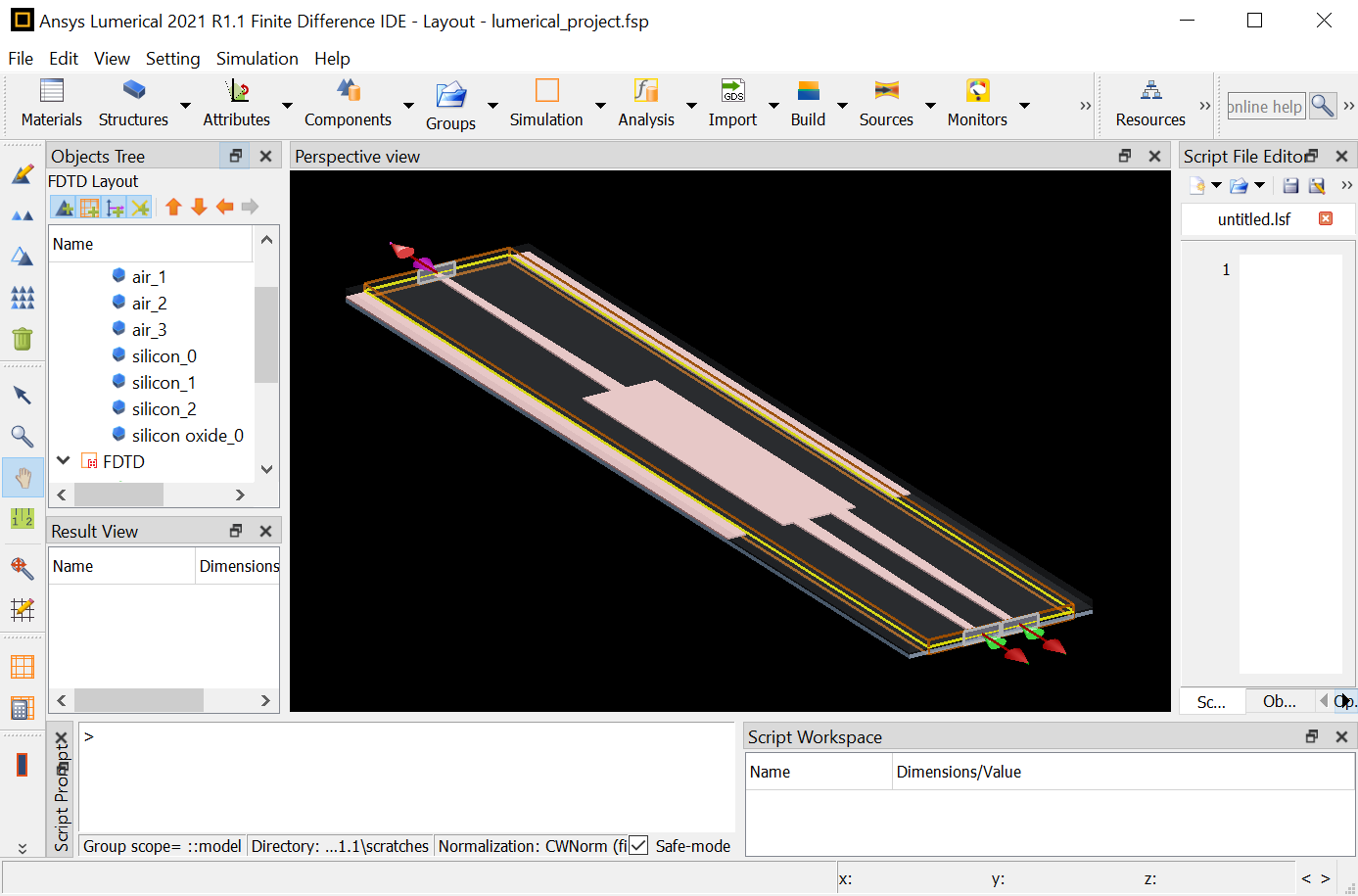
You can now explore the geometry, ports, outputs and other settings as exported by IPKISS. You can make changes and modify settings from here. See Export additional settings below on how to make those settings available for future projects.
4. Retrieve and plot simulation results
After you’ve confirmed that the simulation setup is correct, you can run the simulation and retrieve the results from the outputs. By default you don’t have to launch the simulation explicitly; when you request the results, IPKISS will run the simulation when required.
import numpy as np
smatrix = simulation.get_result(name='smatrix')
transmission = np.abs(smatrix['out1', 'in']) ** 2
Note
By default, the S-matrix that is returned after the simulation will have its sweep units in micrometer.
This is in contrast to manually importing the S-matrix touchstone file using import_touchstone_smatrix,
in which case the default sweep units are in GHz.
Since not all tools use the same physics conventions (e.g. \(\exp(-j\omega t)\) vs \(\exp(j \omega t)\)), IPKISS will ensure that the S-parameters are converted from the tool conventions into IPKISS conventions (\(\exp(-j\omega t)\)).
You can now plot these S-parameters with matplotlib,
or they can be stored to disk (S-parameter data handling).
Lumerical FDTD will also create a touchstone file named ‘smatrix.s3p’ that can be imported using
import_touchstone_smatrix.
import numpy as np
import matplotlib.pyplot as plt
wavelengths = smatrix.sweep_parameter_values
dB = lambda x: 20*np.log10(np.abs(x))
plt.figure()
plt.plot(wavelengths, dB(smatrix["out1", "in"]), label='transmission', linewidth=3, color='g', marker='o')
plt.plot(wavelengths, dB(smatrix["out2", "out1"]), label='crosstalk', linewidth=3, color='b', marker='o')
plt.plot(wavelengths, dB(smatrix["in", "in"]), label='reflection', linewidth=3, color='r', marker='o')
plt.legend()
plt.xlabel('wavelength [$\mu m$]')
plt.ylabel('S-parameter magnitude')
plt.show()
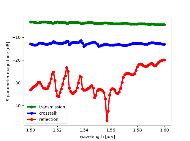
Only the transmission to the ‘out1’ port is plotted because the MMI is symmetric. We see that less than half of the power is transmitted to each output port, so the MMI can be optimized further.
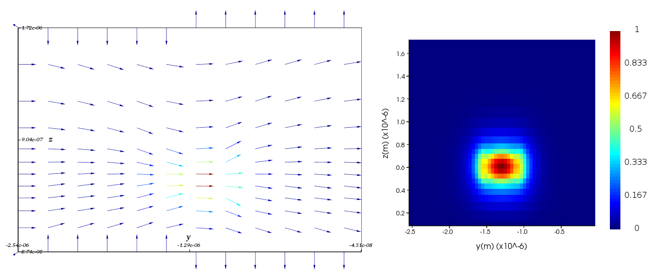
The electric field at the output port can be visualized thanks to the monitor we placed earlier:
5. Advanced simulation settings
Monitors
Just as is the case with the geometry, IPKISS sets reasonable defaults for the port monitors.
When you don’t specify any ports, defaults will automatically be added.
The default position, direction are directly taken from the OpticalPorts of the layout, the dimensions of the Ports are calculated with a heuristic.
Specifically, the width of the port is taken from the core_width attribute of the trace_template of the IPKISS OpticalPort.
Any waveguide template that is a WindowWaveguideTemplate will have this attribute.
For the majority of waveguide templates this is the case. The heuristic will add a fixed margin of 1um to this core_width.
The height of the port is derived from the Material Stack used to virtually fabricate the layer of the core of the Waveguide,
searching for the highest refractive index region but excluding the bottom, top, left and right boundary materials.
You can override these defaults by using the monitors argument of the simulator class:
simulation = i3.device_sim.LumericalFDTDSimulation(
    geometry=sim_geom,
    monitors=[
        i3.device_sim.Port(
            name='in',
            # we make the box of the port quite large for demonstration purposes
            box_size=(5., 5.)
        ),
        i3.device_sim.Port(name='out1'),
        i3.device_sim.Port(name='out2')
    ]
)
When you inspect the simulation object you’ll see something similar to the picture below:
Multimode waveguides
By default, waveguide ports will be simulated with a single mode (the fundamental mode). You can override this in order to take multiple modes into account:
simjob = i3.device_sim.LumericalFDTDSimulation(
   geometry=geometry,
   monitors=[i3.device_sim.Port(name="in", n_modes=2),
             i3.device_sim.Port(name="out1", n_modes=2),
             i3.device_sim.Port(name="out2", n_modes=2)],
   outputs=[
      i3.device_sim.SMatrixOutput(
         name='smatrix',
         wavelength_range=(1.5, 1.6, 100),
         symmetries=[('out1', 'out2')]
      )
   ]
)
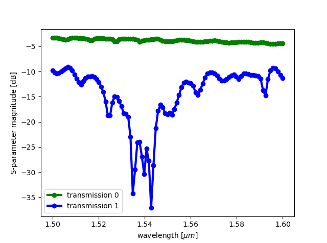
The expectation is that the tool will order the modes according to descending propagation constant, the ground mode being the first mode, the mode with the second largest propagation constant second, and so forth.
The simulation results will then contain the S-parameters for each port-mode combination:
smatrix = simjob.get_result(name='smatrix')

import numpy as np
import matplotlib.pyplot as plt
wavelengths = smatrix.sweep_parameter_values
dB = lambda x: 20*np.log10(np.abs(x))
plt.figure()
plt.plot(wavelengths, dB(smatrix["out1:0", "in:0"]), marker='o', label='transmission 0', linewidth=3, color='g')
plt.plot(wavelengths, dB(smatrix["out1:1", "in:1"]), marker='o', label='transmission 1', linewidth=3, color='b')
plt.legend()
plt.xlabel('wavelength [$\mu m$]')
plt.ylabel('S-parameter magnitude [dB]')
plt.show()
6. Tool-specific settings
In addition to generic settings which can be applied to multiple solvers, the IPKISS device simulation interface also allows to use the full power of the solver tool. Tool-specific materials can be used and tool-specific macros can be defined.
Using materials defined by the simulation tool
By default, IPKISS exports materials for each material used in the process flow definition.
You can also reuse materials which are already defined by the device solvers by
specifying a dictionary solver_material_map to the simulation object
(LumericalFDTDSimulation).
It maps IPKISS materials onto materials defined by the tool (name-based).
For example:
simjob = i3.device_sim.LumericalFDTDSimulation(
    ....
    solver_material_map={
        i3.TECH.MATERIALS.SILICON: 'Si (Silicon) - Palik',
        i3.TECH.MATERIALS.SILICON_OXIDE: 'SiO2 (Glass) - Palik'
    }
)
This will map the TECH.MATERIALS.SILICON, and SILICON_OXIDE, onto materials defined by the electromagnetic solver. The material name should be know by the solver. Please check the tool documentation to find out which materials are available.
Macros
Macros allow you to add tool-specific commands using their API. We have already demonstrated this above by setting the mesh accuracy in Lumerical FDTD.
IPKISS provides some premade macros which are available under the i3.device_sim.lumerical_macros namespace.
Visit the documentation for more information.
You can also use macros to execute tool-specific code to generate output files and retrieve those with simjob.get_result. In the following example we use it to generate a file with the numbers 0 to 5.
simjob = i3.device_sim.LumericalFDTDSimulation(
    geometry=geometry,
    outputs=[
        i3.device_sim.MacroOutput(
            name='macro-output',
            # filepath must correspond with the file used in the commands.
            filepath='test.txt',
            commands=[
                'a=linspace(0, 4, 5);',
                'write("test.txt",num2str(a), "overwrite");'
            ]

        )
    ],
)

# get_result will execute the code and take care of copying the file when required.
fpath = simjob.get_result('macro-ouput')
print(open(fpath).read())
# expected output:
# 0
# 1
# 2
# 3
# 4
Warning
When your lumerical script contains a for loop, you should pass your commands using a multi-line string:
# the following will fail:
output_numbers = i3.device_sim.MacroOutput(
  name="sweep-numbers",
  filepath="numbers.txt",
  commands=[
    'numbers=linspace(0, 4, 5);',
    'for(num=numbers){',
    '  write("numbers.txt", num2str(num));',
    '}'
  ]
)


# instead use a multiline string:
output_numbers = i3.device_sim.MacroOutput(
  name="sweep-numbers",
  filepath="numbers.txt",
  commands=["""
    numbers=linspace(0, 4, 5);
    for(num=numbers){
      write("numbers.txt", num2str(num));
    }
    """
  ]
)
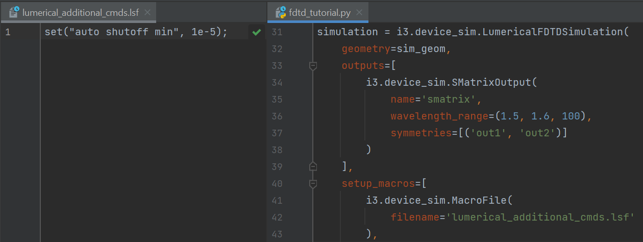
Export additional settings from Lumerical FDTD to IPKISS
Often you will want to tweak certain settings (simulation settings, materials, …) using very tool-specific commands or actions. Since it is not feasible to abstract everything, IPKISS provides a way to store and apply tool-specific settings.
When inspecting the simulation project from the Lumerical FDTD GUI, one can easily tweak any desired settings from the GUI. Almost anything can be modified, really. Consult the Lumerical manual for information.
As an example, we modify the FDTD automatic shutoff value as follows:
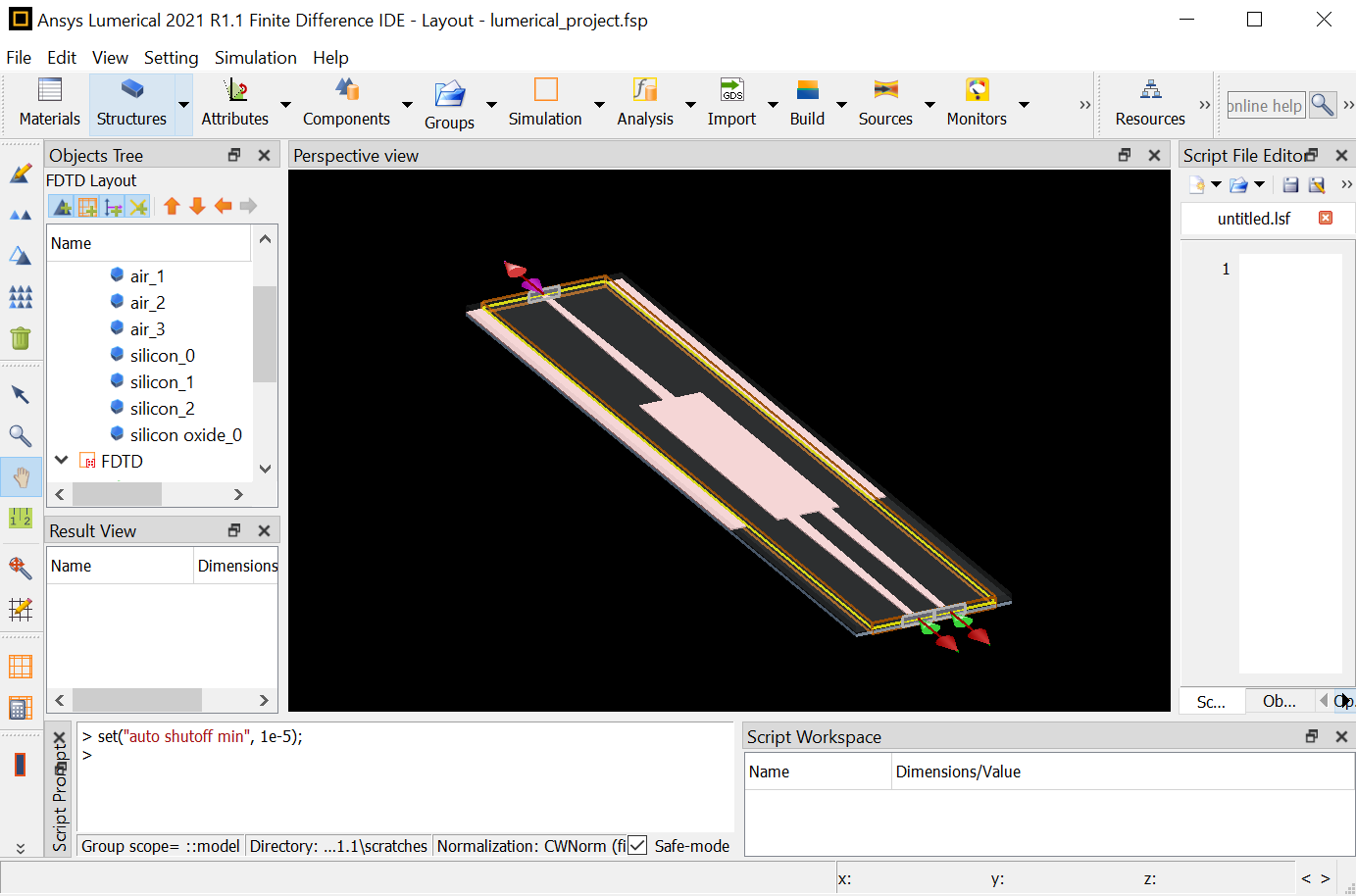
Now, we can store all the additional settings which were made back into the IPKISS model. These will then automatically be re-applied when you run the same simulation next time, also when you make changes to the device geometry, virtual fabrication process or simulation settings!
Save the settings to IPKISS by copying your commands and storing them into a file.