Circuit Simulation with Scatter Matrices
Passive devices can be characterized by their scatter matrix. This scatter matrix can be obtained either by running physical device simulations or by measuring devices on chip.
From this scatter matrix, we can build a circuit model representation. This compact model representation can be efficiently used to simulate circuits with our circuit simulator.
Loading from touchstone into SMatrix1DSweep
A standard format to store these S-matrices is the TouchStone format.
The touchstone file extension typically follows the format ‘sXp’, where X is the number of ports.
If you are not familiar with this format it is recommended to read the Touchstone File Format Specification.
IPKISS has a Touchstone importer (import_touchstone_smatrix)
that loads a touchstone file into an SMatrix1DSweep object.
import ipkiss3.all as i3
import numpy as np
import matplotlib.pyplot as plt
# this how a simple touchstone file looks like
ts_4port = """
! 4-port S-parameter data, taken at three frequency points
# GHZ S MA R 50
5.00000 0.60 161.24 0.40 -42.20 0.42 -66.58 0.53 -79.34 !row 1
0.40 -42.20 0.60 161.20 0.53 -79.34 0.42 -66.58 !row 2
0.42 -66.58 0.53 -79.34 0.60 161.24 0.40 -42.20 !row 3
0.53 -79.34 0.42 -66.58 0.40 -42.20 0.60 161.24 !row 4
6.00000 0.57 150.37 0.40 -44.34 0.41 -81.24 0.57 -95.77 !row 1
0.40 -44.34 0.57 150.37 0.57 -95.77 0.41 -81.24 !row 2
0.41 -81.24 0.57 -95.77 0.57 150.37 0.40 -44.34 !row 3
0.57 -95.77 0.41 -81.24 0.40 -44.34 0.57 150.37 !row 4
7.00000 0.50 136.69 0.45 -46.41 0.37 -99.09 0.62 -114.19 !row 1
0.45 -46.41 0.50 136.69 0.62 -114.19 0.37 -99.09 !row 2
0.37 -99.09 0.62 -114.19 0.50 136.69 0.45 -46.41 !row 3
0.62 -114.19 0.37 -99.09 0.45 -46.41 0.50 136.69 !row 4
"""
# we'll write this to a file with the extension 's4p' because it's a component with 4 ports
with open('simple_test.s4p', 'w') as out:
out.write(ts_4port)
# now we use SMatrix1DSweep to load this file
smat = i3.device_sim.SMatrix1DSweep.from_touchstone('simple_test.s4p')
sweep_values = smat.sweep_parameter_values
unit = smat.sweep_parameter_unit
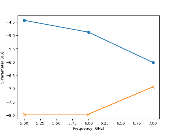
plt.plot(sweep_values, 20 * np.log10(np.abs(smat[0, 0])), 'o-', markersize=7, linewidth=2)
plt.plot(sweep_values, 20 * np.log10(np.abs(smat[0, 1])), 'x-', markersize=7, linewidth=2)
plt.xlabel("Frequency ({})".format(unit))
plt.ylabel("S Parameter [dB]")
plt.show()
Using integers to index the ports can quickly become cumbersome. We want to give names to our ports.
To do this, you can use the term_mode_map argument to tell IPKISS to which port the data in the touchstone file corresponds.
The following example shows how we can add port names to our smatrix by defining the term_mode_map.
# let's assume that our touchstone file represents a
# waveguide with 2 ports, 'in' and 'out'.
# each of these ports has 2 modes.
smat = i3.device_sim.SMatrix1DSweep.from_touchstone(
   'simple_test.s4p',
   term_mode_map={
     ('in', 0): 0,
     ('in', 1): 1,
     ('out', 0): 2,
     ('out', 1): 3,
   }
)

# now we can access the data using the port names:
assert smat['in:0', 'out:0', 0] == smat[0, 2, 0]
# this is the same as:
assert smat['in', 'out', 0] == smat[0, 2, 0]
# to get the TE (mode 0) / TM (mode 1) transmission from in --> out:
assert smat['out:1', 'in:0', 0] == smat[3, 0, 0]
Specific 3rd party tool support
Some 3rd party tools and simulators write metadata to the touchstone file containing among others the port information. When this metadata is available the from_touchstone method will parse it and you don’t need to specify the term_mode_map argument yourself.
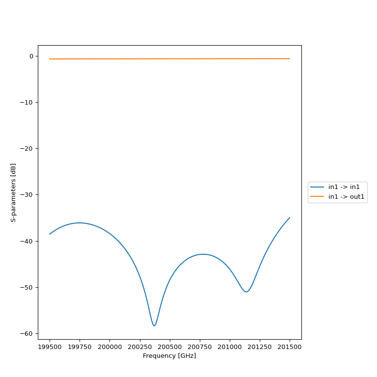
In the following example we load the dircoup.s4p touchstone file generated by a CST Microwave Studio simulation. You can download this dircoup.s4p file here.
import ipkiss3.all as i3
import matplotlib.pyplot as plt
import numpy as np

smat = i3.device_sim.SMatrix1DSweep.from_touchstone("dircoup.s4p")

sweep_values = smat.sweep_parameter_values
unit = smat.sweep_parameter_unit

plt.plot(sweep_values, 20 * np.log10(np.abs(smat["in1", "in1"])), label="in1 reflection")
plt.plot(sweep_values, 20 * np.log10(np.abs(smat["out1", "in1"])), label="in1 -> out1")
plt.xlabel("Frequency ({})".format(unit))
plt.ylabel("S Parameter [dB]")
plt.legend()
plt.show()
The tool-specific importers also convert between the phase convention of the tool and the phase convention of IPKISS. IPKISS uses a \(\exp(j\phi)\exp(-j\omega t)\) conventions but some tools use \(\exp(-j\phi)\exp(j\omega t)\) and hence the S-parameters need to be conjugated in order to use them correctly within IPKISS. The importers for CST Studio Suite ® and Lumerical ensure that the S-parameters can be used directly within IPKISS.
Saving S-matrices to a TouchStone file
A SMatrix1DSweep object can also be saved to a TouchStone file so that it
can be reloaded later.
This can be useful, for example, when you have run long frequency domain simulations, and you want to save the resulting S-parameter data to a file so you do not have to rerun the simulation later on.
Use the to_touchstone method to save the smatrix to a file. The extension, e.g. s3p for a 3-port device, will be added automatically.
s_matrix.to_touchstone("my_smatrix")
s_matrix=i3.device_sim.SMatrix1DSweep.from_touchstone("my_smatrix.s3p")
Example scripts for saving and loading S-parameter data is available here:
It is advised to not save the SMatrix1DSweep object to a binary file with pickle or joblib, since that makes it potentially incompatible across different platforms.
Creating a B-Spline interpolation model
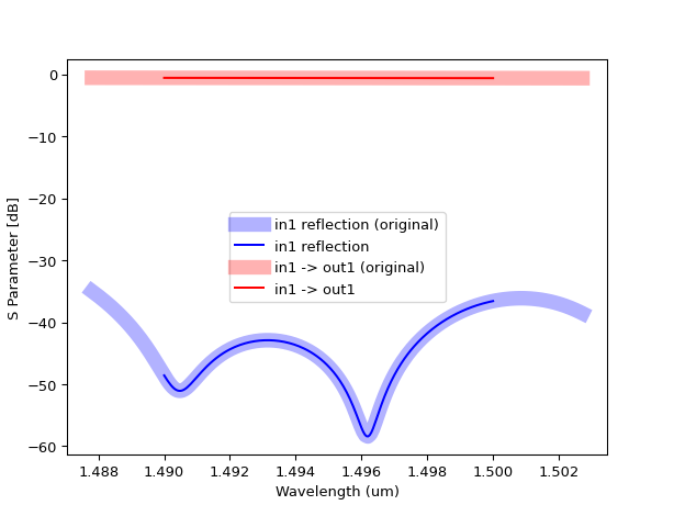
In the previous section we explained how you can load a touchstone file into an SMatrix1DSweep. Now we can easily create an S-model by interpolating
the data in this SMatrix1DSweep object by using the from_smatrix method of the BSplineSModel circuit model class:
"""Creating a directional coupler compact model based on S-parameter data.

"""
import ipkiss3.all as i3
import matplotlib.pyplot as plt
import numpy as np

smat = i3.circuit_sim.SMatrix1DSweep.from_touchstone("dircoup.s4p", unit="um")
bsplinesmodel = i3.circuit_sim.BSplineSModel.from_smatrix(smat, k=3)

# We can quickly check how well the model fits by sampling over a wavelength range
wavelengths = np.linspace(1.49, 1.50, 201)
smat_sim = i3.circuit_sim.test_circuitmodel(bsplinesmodel, wavelengths)

plt.plot(
    smat.sweep_parameter_values,
    20 * np.log10(np.abs(smat["in1", "in1"])),
    "b",
    linewidth=10,
    alpha=0.3,
    label="in1 reflection (original)",
)
plt.plot(wavelengths, 20 * np.log10(np.abs(smat_sim["in1", "in1"])), "b", label="in1 reflection")
plt.plot(
    smat.sweep_parameter_values,
    20 * np.log10(np.abs(smat["out1", "in1"])),
    "r",
    linewidth=10,
    alpha=0.3,
    label="in1 -> out1 (original)",
)
plt.plot(wavelengths, 20 * np.log10(np.abs(smat_sim["out1", "in1"])), "r", label="in1 -> out1")
plt.xlabel("Wavelength (um)")
plt.ylabel("S Parameter [dB]")
plt.legend()
plt.show()
Download the full example here, including the s-parameters: dircoup.s4p.
You might notice that even when the touchstone file contains values in Ghz, the result of the simulation is in wavelengths. When building the model, IPKISS will take care of the unit conversion for you. It will as well ensure that the sweep parameter values are sorted, this is required for interpolation.
When working with measurement data, your data might not be perfect and require preprocessing.
To do so, you can use the modified_copy method to create a copy and modify some of the properties.
You might for example want to prune some sweep values, to reduce the number of coefficients used in the model:
smat_pruned = smat.modified_copy(
    # only select the data every 10 steps
    data=smat.data[:, :, ::10],
    sweep_parameter_values=smat.sweep_parameter_values[::10]
)

bsplinesmodel = i3.circuit_sim.BSplineSModel.from_smatrix(smat_pruned)
To quickly test your model, you can use i3.circuit_sim.test_circuitmodel:
import ipkiss3.all as i3
import numpy as np

wavelengths = np.linspace(1.49, 1.50, 201)
smat = i3.circuit_sim.test_circuitmodel(bsplinesmodel, wavelengths)

assert smat['in1', 'out1'] == smat['out1', 'in1']
Assigning an smatrix model to your PCell
Here’s how to include the generated S-matrix data into your device circuit model view, so it can be used in circuit simulation:
class MyPCell(i3.PCell):
    class Layout(i3.LayoutView):
        #...  here the layout is defined as usual
        pass

    class CircuitModel(i3.CircuitModelView):
        touchstone_filename = i3.StringProperty(default="somefile.s4p", doc="touchstone file, can be from physical simulation or measurement")

        def _generate_model(self):
            smat = i3.circuit_sim.SMatrix1DSweep.from_touchstone(self.touchstone_filename)
            model = i3.circuit_sim.BSplineSModel.from_smatrix(smat, k=3)
            return model