Circuit simulation
Frequency-domain simulation
If every component in a circuit has a model attached to it, running a frequency-domain simulation is quite simple. Let’s start with the two-level splitter tree from the previous chapter as an example. As always, we first import the PDK, IPKISS, and any other dependencies we need:
from si_fab import all as pdk  # noqa: F401
from ipkiss3 import all as i3
import pylab as plt
import numpy as np
from circuits_to_simulate import SplitterTree  # importing the circuit we want to simulate
Because every MMI and waveguide in SiFab has a predefined model already,
we just need to instantiate the CircuitModelView of the circuit and call get_smatrix:
circuit = SplitterTree() # instantiate our basic SplitterTree circuit
circuit_model = circuit.CircuitModel()  # instantiate our SplitterTree circuit model
wavelengths = np.linspace(1.5, 1.6, 501)  # create an array of wavelengths for simulation in units of micrometers
S_total = circuit_model.get_smatrix(wavelengths=wavelengths)
The result is an S-matrix describing the transmission between any two ports, and can be visualized using Matplotlib or a dedicated visualizer. The usage of Matplotlib is shown below. We see that the power is split evenly among the outputs and there are some small reflections at the input.
plt.plot(wavelengths, i3.signal_power_dB(S_total["out1", "in"]), linewidth=2, label="out1")
plt.plot(wavelengths, i3.signal_power_dB(S_total["out2", "in"]), linewidth=2, label="out2")
plt.plot(wavelengths, i3.signal_power_dB(S_total["out3", "in"]), linewidth=2, label="out3")
plt.plot(wavelengths, i3.signal_power_dB(S_total["out4", "in"]), linewidth=2, label="out4")
plt.xlabel(r"Wavelength [$\mu$m]", fontsize=16)  # add a label to the x-axis
plt.ylabel("Transmission [dB]", fontsize=16)
plt.ylim([-10, 0])
plt.legend(fontsize=14)  # create a legend from the plt.plot labels
plt.show()  # show the graph
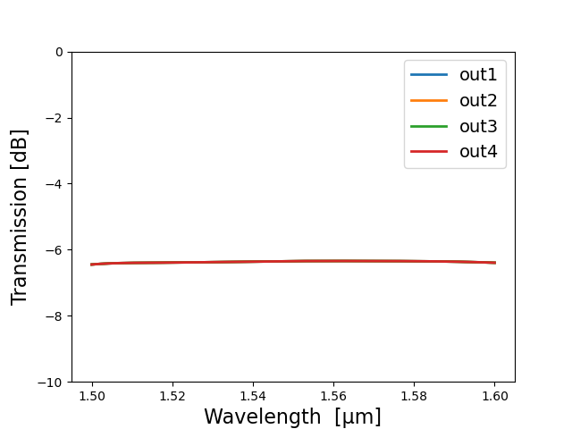
Frequency-domain simulation of a two-level splitter tree design: transmission
An easier way to plot the results of an S-matrix frequency sweep is to use a dedicated visualize method.
    S_total.visualize(
        term_pairs=[("in", "out1"), ("in", "out2"), ("in", "out3"), ("in", "out4")],
        scale="dB",
        ylabel="Transmission [dB]",
        yrange=(-10.0, 0.0),
        figsize=(9, 5),
    )
    S_total.visualize(
        term_pairs=[("in", "in")],
        scale="dB",
        ylabel="Reflection [dB]",
        yrange=(-80.0, -30.0),
        figsize=(9, 5),
    )
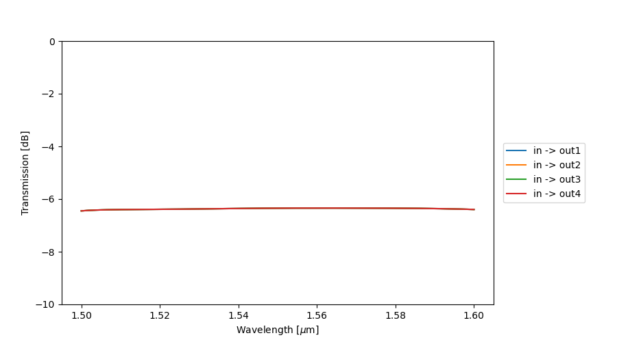
Frequency-domain simulation of a two-level splitter tree design: transmission
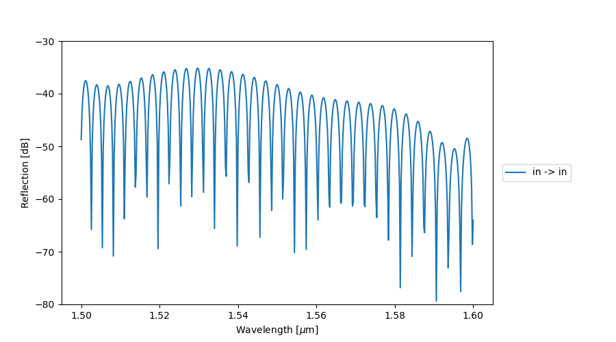
Frequency-domain simulation of a two-level splitter tree design: reflection
Running these simulations in a code environment provides interesting possibilities. We can, for example, use for-loops to sweep a parameter’s value and find out how it impacts the circuit’s performance. This can be demonstrated with a Mach-Zehnder Interferometer (MZI):
mzi = MZI(path_difference=100)
mzi_layout = mzi.Layout()
mzi_layout.visualize(annotate=True)
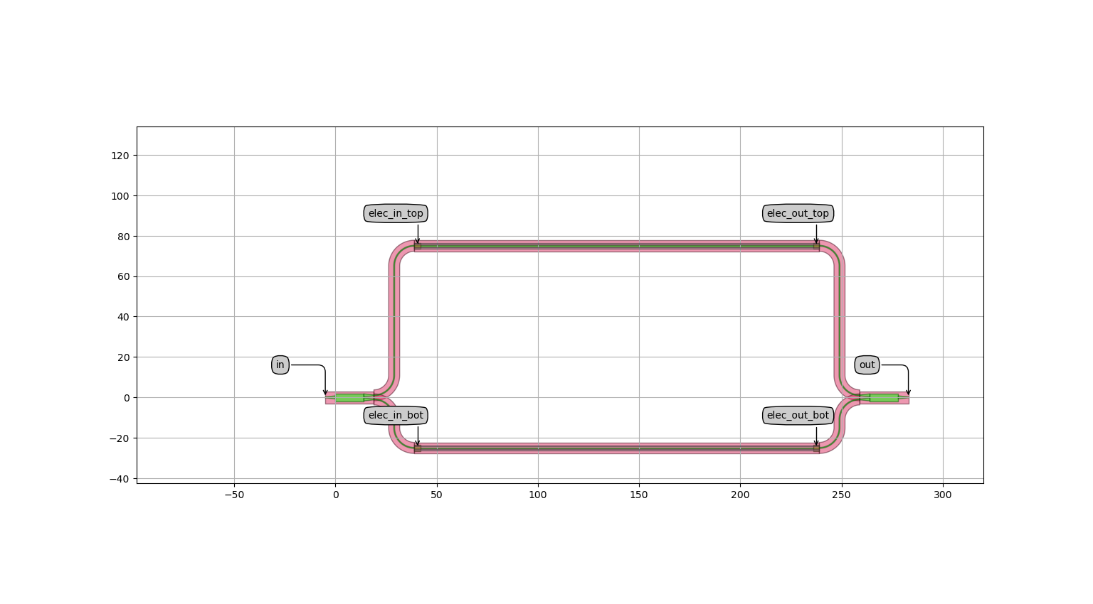
Mach-Zehnder Interferometer with heated top and bottom arm
We will sweep over a range of path length differences between the two arms of the MZI, resulting in different interference patterns at the output:
path_differences = np.linspace(50, 150, 3) # range from 50 to 150 um, in steps of 50 um
for path_difference in path_differences:  # iterate over "path_differences"
    mzi_model = MZI(path_difference=path_difference).CircuitModel()  # call the CircuitModel() method on each new MZI
    mzi_model.get_smatrix(wavelength_range).visualize(  # calculate and visualize the s_matrix
        term_pairs=[("in", "out")],
        scale="dB",  # convert to dB
        ylabel="Transmission [dB]",
        yrange=(-60.0, 0.0),
        title=f"path_difference = {path_difference}",  # use f-strings to format the title
        figsize=(9, 5),
    )
Similar to the first example, the result for each value of the path length difference can be plotted. As the path difference increases, the free spectral range decreases proportionally as expected.
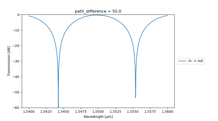
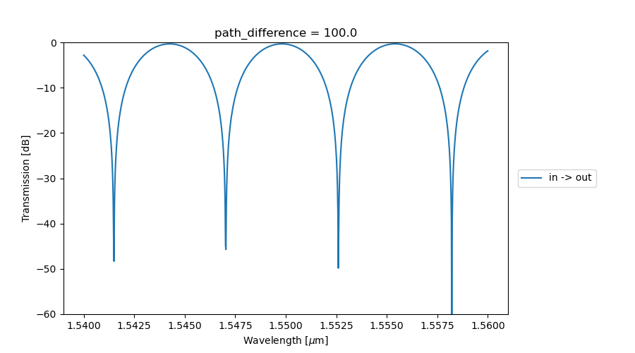
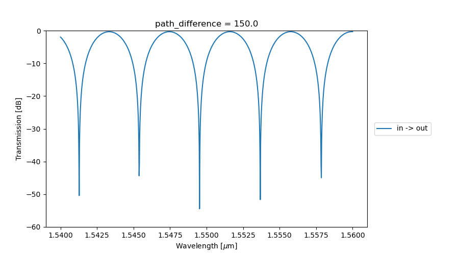
MZI transmission as a function of path difference between the top and bottom arm
Time-domain simulation
To conclude, we’ll have a short look at time-domain simulations. These are slightly more complicated than frequency-domain simulations, and fully describing them is out of the scope of a ‘getting started’ course. If you want more information, please visit Creating a First Circuit Simulation.
Both arms of the MZI in the previous example can be thermally tuned by applying a voltage to their electrical ports. If a constant optical signal is sent through the input while the voltage across one of the arms is steadily increased, we expect that the power level at the output will change over time. To test this, let’s start by creating optical and electrical sources:
def ramp_function(t_rise, amplitude):
    """Returns a simple linear voltage ramping function to apply to our circuit. "t" is the current time in the
    simulation, "t_rise" is the time it takes for the voltage to ramp to its maximum, and "amplitude" is the final
    value of the applied voltage.
    """

    def f_step(t):
        if t <= t_rise:
            return amplitude * (t / t_rise)
        else:
            return amplitude

    return f_step
dt = 1e-7  # setting up the time step variable for our simulation
voltage_function = ramp_function(t_rise=70 * dt, amplitude=3.5)  # create our driving voltage function
optical_source = i3.FunctionExcitation(port_domain=i3.OpticalDomain, excitation_function=lambda x: 1)
voltage_drive = i3.FunctionExcitation(port_domain=i3.ElectricalDomain, excitation_function=voltage_function)
Next, similarly to what you would do in a real lab setting, we will create a virtual ‘testbench’ circuit that connects the MZI to the sources and a probe to register the transmission at the output.
To make these logical connections we can use i3.ConnectComponents:
circuit = i3.ConnectComponents(
    child_cells={
        "mzm": MZI(path_difference=5.5),  # the circuit we want to simulate
        "src_opt": optical_source,  # the optical source to be used
        "v_drive": voltage_drive,  # the drive voltage excitation
        "opt_out_probe": i3.Probe(port_domain=i3.OpticalDomain),  # our optical monitor
    },
    links=[
        ("v_drive:out", "mzm:elec_in_bot"),  # connect the dc_voltage to one of the electric heaters in the circuit
        ("src_opt:out", "mzm:in"),  # connect the optical source to the MZI optical input
        ("mzm:out", "opt_out_probe:in"),  # connect the optical probe to the MZI optical output
    ],
)
As you can see, the voltage is applied to the bottom arm. The source and probe are connected to the input and output of the MZI respectively.
Finally, we instantiate the CircuitModelView and call get_time_response,
passing in our parameters for the start and end times, time step and central wavelength:
result = circuit.CircuitModel().get_time_response(t0=0.0, t1=1e-5, dt=dt, center_wavelength=1.55)
Plotting the result can be done in the following way:
plt.title("MZI thermal tuning in the time domain", size=20)
plt.xlabel("Simulation time steps")
plt.ylabel("Optical output power [dB]")
plt.plot(i3.signal_power_dB(result["opt_out_probe"][1:]))
plt.show()
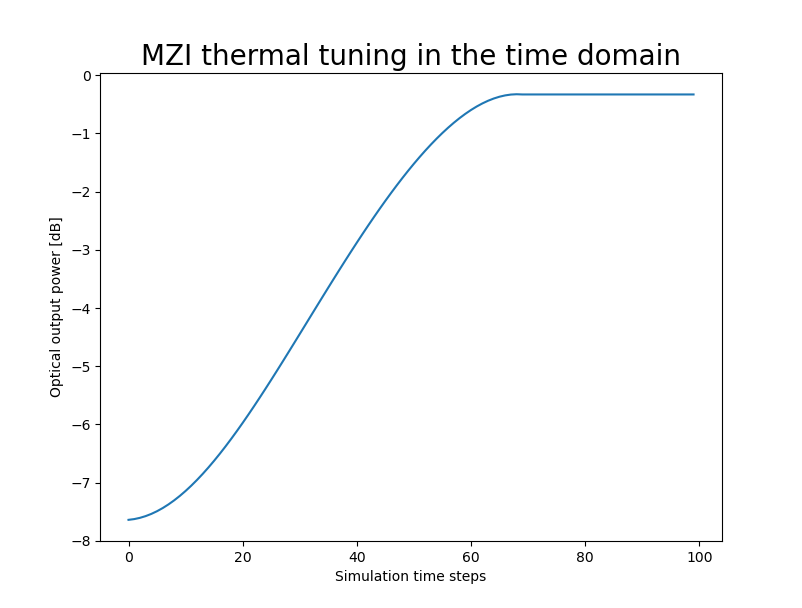
Time-domain simulation of a thermally tuned MZI
As expected, we see the initial transmission is poor due to the imbalance in the path differences. As we apply our ramping voltage, the refractive index in the bottom arm changes, reducing the phase difference and resulting in a higher overall transmission.
More information
We have purposely left out what the models of our components look like and how to implement them. This is covered in a later section of the “getting started” course: Component Models.
Find out what Caphe has to offer and what its advantages are: Caphe introduction.
Exercise
In getting_started/4_circuit_simulation/2_exercises/exercises.py you will find an incomplete Python script. The purpose of the script is to run a frequency-domain simulation of a circuit with and without grating couplers. To practice what we’ve learned in this chapter, try to fill in the missing code. There is also a solution file in case you get stuck.