AWG generation: Synthesis
Now that we have established and reviewed the subcomponents (slab template, apertures and waveguide model), we can start the synthesis of the AWG.
We will formulate the high-level specifications and translate them into AWG implementation parameters. The inputs required are:
The functional specifications: center frequency, number of channels, channel spacing, FSR, …
The subcomponents: slab template, apertures, waveguide template
Some independent physical specifications that impact optical performance, such as the minimum spacing of the output waveguides
Note
The synthesis algorithm used here is provided by the Luceda AWG Designer and reflect best design practices. It is possible to write your own synthesis algorithm if finer control is needed.
Functional specifications
The next step is to define your functional specifications, fab rules and optical rules. This means you need to choose the free spectral range, channel spacing, and several layout parameters for the apertures, grating pitch, and so on. Based on this, the AWG devices are synthesized: implementation parameters are derived, such as angles, positions, radii, delay length.
The two images below summarize the required information. In yellow are the inputs. In grey are the outputs.
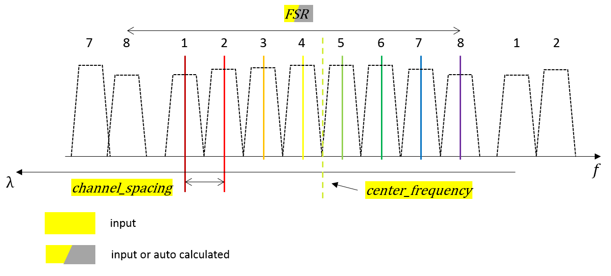
The target application uses 8 channels centered around 232.2 THz frequency. The channels are spaced 800 GHz, except around the center where the center frequency itself is not used.

In this example, we will keep the center channel at 232.2 THz and use it as a monitor output of the AWG. Therefore, we will synthesize the AWG with 9 channels.
Channels
Since we have an AWG with equidistantly spaced frequency channels, we will start by specifying the center frequency, the channel spacing (in Hz) and an array of channel frequencies. Because we will use the center channel as a monitor, we have included it in the specifications.
Free Spectral Range
A second specification is the free spectral range (FSR) of the device. Since this device functions as a demultiplexer and we only utilize one FSR, we make the FSR wider than the span of the channels. This is beneficial so as to reduce the insertion loss non-uniformity. If we had chosen the FSR equal to the number of channels times their spacing, the outer channels would incur about 3 dB of excess loss compared to the center channel, as predicted from AWG theory. If we increase the FSR, the channels will be more uniform. However, if we make the FSR very large, the delay length between the waveguides will become increasingly small, to the extent that it may be difficult to route the waveguide array.
For this reason, here we choose to make the FSR parametric so that benefits and drawbacks of increasing the FSR can be balanced against eachother.
We define the functional specifications near the top of our script as shown below:
# Set your desired center frequency.
center_frequency = 232200.0  # units in GHz

# Set the desired spacing between wavelength channels.
channel_spacing = 800.0  # units in GHz

# Set your desired number of wavelength channels:
n_channels = 9

# Set your desired Free Spectral Range.
fsr = 10400
Physical specifications
Now we need to supply a few physical specifications to the synthesis algorithm.
The first specification is how wide we want the angular coverage of the waveguide array to be. This is expressed as an alpha factor parameter, by which the \(1/e^2\) optical beam divergence angle in the star coupler is multiplied. Typically, a value of 1.4-1.6 is used to ensure nearly all diffracted light is captured by the waveguide array.
The second specification is how far we want the output apertures to be spaced. A spacing that is too small will give rise to crosstalk. We prefer the apertures to be sufficiently decoupled, so we want to make this spacing large enough. However, a larger spacing will also require the star coupler to become larger (with constant angular dispersion by the grating and free propagation region). The output spacing chosen will therefore not only affect nearest neighbour crosstalk but also set a minimum for the star coupler diameter. In this case, we choose a minimum center-to-center spacing of 7 um, which should be enough to decouple apertures with a width of 2 um.
Another specification that you can provide is the number of arms. In this case, we set it to None to have it set automatically.
# Minimum spacing between the output apertures (center-to-center).
# Increasing this value means less crosstalk but more power lost between the two channels.
output_aperture_spacing = 7.0

# This value affects the angular spread of the output apertures.
fpr_alpha_factor = 1.6

# Set your desired number of arrayed waveguide arms.
# Default is None for an automatic number of arms.
n_arms = None
Subcomponents
Next, we instantiate the subcomponents. We have already reviewed their definition and model in the previous step, thus we simply construct them.
print("Instantiating subcomponents...\n")

# Use the slab template from PDK.
slab = SiSlabTemplate()

# Calculate the slab modes with CAMFR.
slab_modes = slab.SlabModesFromCamfr(wavelengths=simulation_wavelengths_slab)

# Use aperture templates from the PDK. We use a standard rib aperture for the outputs and arms.
aperture = SiRibAperture(slab_template=slab, wire_width=wg_width)

# Simulate the aperture at only the center length to save on computation time.
aperture.CircuitModel(simulation_wavelengths=[center_wavelength])

# You can use an MMI aperture for the input. This creates a broad transmission band for the frequency channels.
aperture_mmi = SiRibMMIAperture(slab_template=slab, wire_width=wg_width)
aperture_mmi.CircuitModel(simulation_wavelengths=[center_wavelength])

# Use the waveguide template from the PDK
wg_tmpl = pdk.SiWireWaveguideTemplate()
wg_tmpl.Layout(core_width=wg_width)
In this case, the waveguide width was also defined as a parameter.
Automated Synthesis
Now that all the necessary inputs are generated, we are ready to derive the implementation parameters.
For an equifrequency channel design, this is done using the get_layout_params_1xM_demux_ghz function in the Luceda AWG Designer.
This function goes through the whole process of deriving low-level implementation parameters from the functional specifications, subcomponents and physical specifications.
print("\nDeriving implementation parameters...\n")

design_params = awg.get_layout_params_1xM_demux_ghz(
    aperture_in=aperture,
    aperture_arms=aperture,
    aperture_out=aperture,
    waveguide_template=wg_tmpl,
    output_spacing=output_aperture_spacing,
    alpha_factor=fpr_alpha_factor,
    M=n_channels,
    center_frequency=center_frequency,
    channel_spacing=channel_spacing,
    FSR=fsr,
    N_arms=n_arms,
    verbose=True,
)
In addition to returning a Python dictionary with implementation parameters, the synthesis function also prints the relevant parameters and calculations:
Data extracted from slab / waveguide model
------------------------------------------
Channels (in um): [ 1.30913737  1.30457989  1.30005402  1.29555946  1.29109586  1.28666291 1.2822603   1.27788772  1.27354485]
Channels (in GHz): [ 229000.  229800.  230600.  231400.  232200.  233000.  233800.  234600. 235400.]
Effective indices of the waveguide at channels: [array(2.566451906841001), array(2.572459055828688), array(2.5784135232713354), array(2.5843160589299594), array(2.59016721323884), array(2.595967488320401), array(2.6017174289497054), array(2.607417596940138), array(2.6130685399918905)]
Effective index at center wavelength: 2.59016721324
Waveguide group index at center wavelength: 4.28105602782
Effective index of the slab at channels: [ 2.99574066  2.99848965  3.00122092  3.00393478  3.00663138  3.00931078 3.01197315  3.01461861  3.01724732]
Calculated aperture period for the grating = 2.2 um
Radius for input circle: 478.646859193 um (same as R_grating because use_same_radius=True)
Actual delay length (using delay_length_from_FSR): 6.47998556057 um
Specified FSR = 10400.0 GHz
FSR (after snapping the delay length, and approximated at center frequency) = 10806.7661344 GHz
f_min: 227000.0, f_max: 237400.0
Spreading angle of the output aperture (alpha_out) = 36.713402734 degrees
Radius for grating circle of the output star coupler (using get_R_grating): 478.646859193 um
Number of grating elements: 139
Effective # channels in actual FSR = 13.508457668
Angles for the outputs: [ -3.37690610e+00  -2.51997833e+00  -1.67172484e+00  -8.31829409e-01 -3.16175780e-14   8.24040859e-01   1.64056203e+00   2.44982305e+00 3.25207306e+00] (degrees)
You can also use get_layout_params_1xM_demux_um if you want an equiwavelength design.
Parameters review
The design_params returned by the Luceda AWG Designer are:
delay_length: delay length between consecutive waveguidesR_grating: the radius of the grating circle at the output star couplerR_input: the radius of the grating circle at the input star couplerN_arms: number of arms in the waveguide arrayangles_arms_out: angles of the waveguide array apertures at the output star couplerangles_out: angles of the output apertures (at the output star coupler)angles_arms_in: angles of the waveguide array apertures at the input star coupler
We can easily review them by printing the design_params dictionary:
# Print output
print("\nDesign parameters:\n")

if plot:
    print(design_params)


# Saving design parameters
{'delay_length': 6.479985560573094,
 'N_arms': 140,
 'R_grating': 478.64685919236774,
 'R_input': 478.64685919236774,
 'angles_arms_in': array([
     -18.62919414, -18.35151102, -18.07427361, -17.79747331,
     -17.52110162, -17.24515016, -16.96961065, -16.69447491,
     -16.41973484, -16.14538246, -15.87140986, -15.59780923,
     -15.32457285, -15.05169308, -14.77916235, -14.5069732 ,
     -14.23511822, -13.96359007, -13.69238152, -13.42148538,
     -13.15089453, -12.88060194, -12.61060062, -12.34088365,
     -12.07144419, -11.80227543, -11.53337064, -11.26472314,
     -10.99632629, -10.72817354, -10.46025835, -10.19257425,
      -9.92511481,  -9.65787367,  -9.39084448,  -9.12402096,
      -8.85739685,  -8.59096595,  -8.32472209,  -8.05865914,
      -7.79277101,  -7.52705164,  -7.26149499,  -6.99609509,
      -6.73084596,  -6.46574168,  -6.20077634,  -5.93594407,
      -5.67123901,  -5.40665534,  -5.14218726,  -4.87782899,
      -4.61357477,  -4.34941886,  -4.08535556,  -3.82137914,
      -3.55748394,  -3.29366429,  -3.02991452,  -2.76622901,
      -2.50260211,  -2.23902822,  -1.97550173,  -1.71201704,
      -1.44856857,  -1.18515072,  -0.92175792,  -0.6583846 ,
      -0.3950252 ,  -0.13167414,   0.13167414,   0.3950252 ,
       0.6583846 ,   0.92175792,   1.18515072,   1.44856857,
       1.71201704,   1.97550173,   2.23902822,   2.50260211,
       2.76622901,   3.02991452,   3.29366429,   3.55748394,
       3.82137914,   4.08535556,   4.34941886,   4.61357477,
       4.87782899,   5.14218726,   5.40665534,   5.67123901,
       5.93594407,   6.20077634,   6.46574168,   6.73084596,
       6.99609509,   7.26149499,   7.52705164,   7.79277101,
       8.05865914,   8.32472209,   8.59096595,   8.85739685,
       9.12402096,   9.39084448,   9.65787367,   9.92511481,
      10.19257425,  10.46025835,  10.72817354,  10.99632629,
      11.26472314,  11.53337064,  11.80227543,  12.07144419,
      12.34088365,  12.61060062,  12.88060194,  13.15089453,
      13.42148538,  13.69238152,  13.96359007,  14.23511822,
      14.5069732 ,  14.77916235,  15.05169308,  15.32457285,
      15.59780923,  15.87140986,  16.14538246,  16.41973484,
      16.69447491,  16.96961065,  17.24515016,  17.52110162,
      17.79747331,  18.07427361,  18.35151102,  18.62919414
 ]),
 'angles_arms_out': array([
      18.62919414,  18.35151102,  18.07427361,  17.79747331,
      17.52110162,  17.24515016,  16.96961065,  16.69447491,
      16.41973484,  16.14538246,  15.87140986,  15.59780923,
      15.32457285,  15.05169308,  14.77916235,  14.5069732 ,
      14.23511822,  13.96359007,  13.69238152,  13.42148538,
      13.15089453,  12.88060194,  12.61060062,  12.34088365,
      12.07144419,  11.80227543,  11.53337064,  11.26472314,
      10.99632629,  10.72817354,  10.46025835,  10.19257425,
       9.92511481,   9.65787367,   9.39084448,   9.12402096,
       8.85739685,   8.59096595,   8.32472209,   8.05865914,
       7.79277101,   7.52705164,   7.26149499,   6.99609509,
       6.73084596,   6.46574168,   6.20077634,   5.93594407,
       5.67123901,   5.40665534,   5.14218726,   4.87782899,
       4.61357477,   4.34941886,   4.08535556,   3.82137914,
       3.55748394,   3.29366429,   3.02991452,   2.76622901,
       2.50260211,   2.23902822,   1.97550173,   1.71201704,
       1.44856857,   1.18515072,   0.92175792,   0.6583846 ,
       0.3950252 ,   0.13167414,  -0.13167414,  -0.3950252 ,
      -0.6583846 ,  -0.92175792,  -1.18515072,  -1.44856857,
      -1.71201704,  -1.97550173,  -2.23902822,  -2.50260211,
      -2.76622901,  -3.02991452,  -3.29366429,  -3.55748394,
      -3.82137914,  -4.08535556,  -4.34941886,  -4.61357477,
      -4.87782899,  -5.14218726,  -5.40665534,  -5.67123901,
      -5.93594407,  -6.20077634,  -6.46574168,  -6.73084596,
      -6.99609509,  -7.26149499,  -7.52705164,  -7.79277101,
      -8.05865914,  -8.32472209,  -8.59096595,  -8.85739685,
      -9.12402096,  -9.39084448,  -9.65787367,  -9.92511481,
     -10.19257425, -10.46025835, -10.72817354, -10.99632629,
     -11.26472314, -11.53337064, -11.80227543, -12.07144419,
     -12.34088365, -12.61060062, -12.88060194, -13.15089453,
     -13.42148538, -13.69238152, -13.96359007, -14.23511822,
     -14.5069732 , -14.77916235, -15.05169308, -15.32457285,
     -15.59780923, -15.87140986, -16.14538246, -16.41973484,
     -16.69447491, -16.96961065, -17.24515016, -17.52110162,
     -17.79747331, -18.07427361, -18.35151102, -18.62919414
 ]), 'angles_out': array([
     -3.37690610e+00, -2.51997833e+00, -1.67172484e+00,
     -8.31829409e-01, -3.16175780e-14,  8.24040859e-01,
      1.64056203e+00,  2.44982305e+00, 3.25207306e+00
 ])}
Storing the result
In addition to visualizing them, we can also store these parameters in a file for later use. Using the JSON package, we can save the data in a platform-independent but human-readable format:
# Saving design parameters
def serialize_ndarray(obj):
    return obj.tolist() if isinstance(obj, np.ndarray) else obj


json_path = os.path.abspath(os.path.join(save_dir, "design_params.json"))
with open(json_path, "w") as f:
    json.dump(design_params, f, sort_keys=True, default=serialize_ndarray, indent=0)
print(f"{json_path} written")
Conclusion
Using the functionality provided by the Luceda AWG Designer, we have synthesized the AWG parameters from functional specifications, subcomponent models and a few physical specifications. In the next step, the derived implementation parameters will be turned into a complete AWG, with a layout and a circuit model.