Note
Go to the end to download the full example code
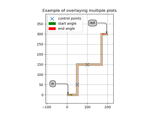
Overlaying multiple plots
It’s possible to extend a visualization generated by IPKISS and add your own information using matplotlib. The example below demonstrates how to create a figure and reuse it to overlay three different plots.
import si_fab.all as pdk
import ipkiss3.all as i3
import pylab as plt


trace_template = pdk.M1WireTemplate()
trace_template.Layout(width=10)

# Create the main figure
fig = plt.figure()
plt.title("Example of overlaying multiple plots")

# Create ports
electrical_in = i3.ElectricalPort(name="in", position=(0, 0), trace_template=trace_template)
electrical_out = i3.ElectricalPort(name="out", position=(200, 300), trace_template=trace_template)

# Create and plot some control points
control_points = [(50, 50), (100, 150)]
cp_plot = plt.scatter(*zip(*control_points), marker="x", s=100, label="control points")

# Add an electrical wire to the figure. show=False since we are still going to add things to our plot.
wire = i3.Circuit(
    specs=[
        i3.ConnectElectrical(
            electrical_in,
            electrical_out,
            start_angle=0,
            end_angle=180,
            control_points=control_points,
            min_straight=25,
            trace_template=trace_template,
        ),
    ],
    exposed_ports={"intermediate_in_to_intermediate_out:in": "in", "intermediate_in_to_intermediate_out:out": "out"},
)
wire.Layout().visualize(figure=fig, annotate=True, show=False)

# Overlay the figure with arrows indicating the start and end angle
plt.arrow(0, 0, 20, 0, width=2, label="start angle", color="green")
plt.arrow(200, 300, -20, 0, width=2, label="end angle", color="red")

# Finally show everything
plt.legend(loc="upper left")
plt.show()