Placement and Routing Reference
An important aspect of building a circuit layout is the placement and routing of cells.
In IPKISS, this is done using i3.Circuit.
This placement and routing function works by choosing a set of instances, and defining specifications (placement, joining, alignment, how to connect, …) that describe how these instances should be placed and connected. The different specifications for placement and routing are listed below.
Functions and classes
The main class to use for building circuits is i3.Circuit. It is an easy-to-use class built around the core algorithm i3.place_and_route, which performs the placement and routing in the layout view.
i3.Circuit also uses i3.NetlistFromLayout, so that the netlist is automatically extracted from the layout. This enables layout-accurate circuit simulations.
Function to place and route a series of instances with the help of placement specifications and connectors. |
A PCell which derives its layout, netlist and model from a set of specifications in order to create a circuit. |
|
Parametric Cell for logically connecting multiple components. |
Specifications
The placement specifications are the following:
Join instances together. |
|
Specifies that an instance ( |
|
(deprecated) Specifies that an instance (inst1) or a port (inst1:port) should be placed relative to another instance (inst2) or a port (inst2:port) with a given offset (x, y) and an angle (optional). |
|
Specifies that instances or ports should be aligned horizontally. |
|
Specifies that instances or ports should be aligned vertically. |
|
Specifies that a horizontally mirrored version of the component must be placed. |
|
Specifies that a vertically mirrored version of the instance must be placed. |
Note
Always be as specific as possible when providing the placement specifications. The placement engine will change the positions of instances that are specified in the specifications list.
For instance, if you have multiple specs without using Place, that tells the placement engine that the location of the full circuit (or at least that one instance) is not important. The instances will still be placed relative to each other as specified, but their position might change when you add more specs. By using Place, you anchor your circuit.
The routing specifications are the following:
Scalar connectors
Base class for connectors. |
|
A connector that uses |
|
A connector that uses |
|
Connector for creating an as simple as possible bend between two optical ports based on the given rounding parameters. |
|
A connector that uses |
Bundle connectors
Connects multiple ports together using a bundle of waveguides separated by a fixed distance. |
|
Connects multiple ports together using a bundle of electrical wires separated by a fixed distance. |
Fanouts for Bundle connectors
Create S-bend-like routes that fanout all the start ports to evenly spaced outputs. |
|
Create L-bend-like routes that fanout all the start ports to evenly spaced outputs. |
Symbols
While doing placement and routing, positions or values are often only known relative to an other instance or port. To avoid tedious calculations, you can use symbols or strings to represent these unknowns and IPKISS will fill in the appropriate values.
The i3.Place specification and control points / lines support this through the relative_to argument:
“inst” signifies the origin point of the instance labeled “inst”.
“inst:out” indicates the position of the “out” port of the instance named “inst”.
“inst@N” denotes the northernmost y-coordinate of the bounding box of the “inst” instance. Other identifiers in this category include E for east, S for south, W for west, C for center and combinations like NE, NW, SE, SW.
For routing purposes, the following symbols can also be used to perform basic arithmetic:
Symbolic object that represents a start value or position. |
|
Symbolic object that represents an end value or position. |
|
Symbolic object that represents a previous value or position. |
For examples on how to use these symbols, visit the documentation pages of the relevant specs and control points / lines.
Route control
Argument control points of connector should be a list. Elements of the control points list can be related to the following:
Description of where a route should pass through. |
|
Horizontal control point class. |
|
Vertical control point class. |
|
Place a via and change trace template at a certain point along the route. |
Control points
Control points i3.CP allow you to specify certain points through which the route should go.
Description of where a route should pass through. |
import si_fab.all as pdk
import ipkiss3.all as i3
import matplotlib.pyplot as plt
fc = pdk.FC_TE_1550()
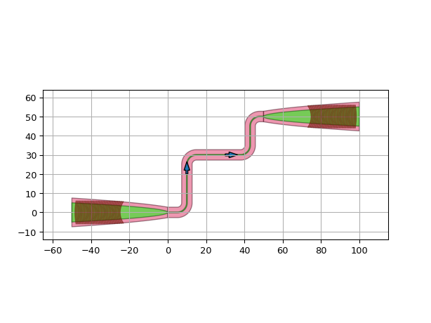
circuit = i3.Circuit(
insts={"fc_in": fc, "fc_out": fc},
specs=[
i3.Place("fc_in:out", position=(0, 0)),
i3.Place("fc_out:out", position=(50, 50)),
i3.FlipH("fc_out"),
i3.ConnectManhattan(
"fc_in:out",
"fc_out:out",
control_points=[i3.CP((10, 20), i3.NORTH), i3.CP((30, 30), i3.EAST)],
),
],
)
circuit.Layout().visualize(show=False)
plt.arrow(10, 20, 0, 2, width=1.0)
plt.arrow(30, 30, 2, 0, width=1.0)
plt.show()
import si_fab.all as pdk # noqa
import ipkiss3.all as i3
from picazzo3.fibcoup.curved.cell import FiberCouplerCurvedGrating
import matplotlib.pyplot as plt
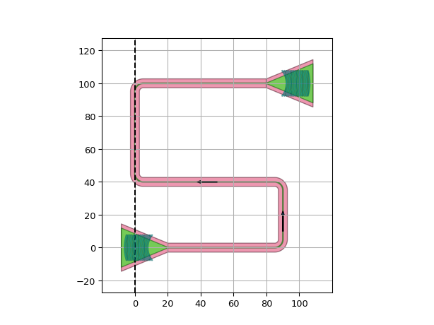
gc = FiberCouplerCurvedGrating()
circuit = i3.Circuit(
insts={"gc_in": gc, "gc_out": gc},
specs=[
i3.Place("gc_in", (0, 0)),
i3.Place("gc_out", (100, 100), angle=180),
i3.ConnectManhattan(
"gc_in:out",
"gc_out:out",
control_points=[
i3.CP((90, 10), i3.NORTH),
i3.CP((50, 40), i3.WEST),
i3.CP((0, None)),
],
),
],
)
circuit.get_default_view(i3.LayoutView).visualize(show=False)
plt.arrow(90, 10, 0, 10, width=0.5)
plt.arrow(50, 40, -10, 0, width=0.5)
plt.axvline(0, color="k", linestyle="--")
plt.show()
Horizontal and Vertical control lines
i3.ConnectManhattan and i3.RouteManhattan allow the definition of horizontal and vertical control lines.
Horizontal control point class. |
|
Vertical control point class. |
i3.H and i3.V represent Horizontal and Vertical lines on a grid.
They are a special case of the more general i3.CP control points,
requiring you to only specify an X-value for i3.V and a Y-value for i3.H:
i3.CP((None, 10)) == i3.H(10)
i3.CP((10, None)) == i3.V(10)
Note
When supplying i3.H and i3.V as control lines they have to be alternated as the lines should cross each other in the order you want the routing to go.
Below are some examples using i3.ConnectManhattan:
An example showing the syntax:
from ipkiss3 import all as i3

control_points = [i3.V(10), i3.H(40), i3.V(35)]

connector = i3.ConnectManhattan('inst1:out', 'inst2:out', control_points=control_points)
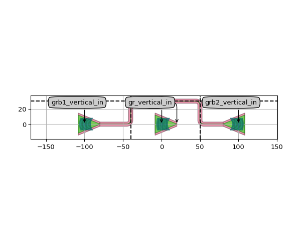
An example showing the usage in an obstacle avoidance situation:
import si_fab.all as pdk
from ipkiss3 import all as i3
from picazzo3.fibcoup.curved import FiberCouplerCurvedGrating
import matplotlib.pyplot as plt

# Placing the components in a circuit
gr = FiberCouplerCurvedGrating()
control_points = [i3.V(-40), i3.H(30), i3.V(50)]
circuit = i3.Circuit(
    insts={
        'gr': gr,
        'grb1': gr,
        'grb2': gr
    },
    specs=[
        i3.Place('gr', position=(0, 0)),
        i3.Place('grb1', position=(-100, 0)),
        i3.Place('grb2', position=(+100, 0), angle=180),

        i3.ConnectManhattan(
            'grb1:out', 'grb2:out',
            control_points=control_points,
        )
    ]
)

lay = circuit.Layout()
lay.visualize(annotate=True, show=False)

plt.axvline(x=-40, color='k', linestyle='--')
plt.axhline(y=30, color='k', linestyle='--')
plt.axvline(x=50, color='k', linestyle='--')
plt.show()
Relative route control
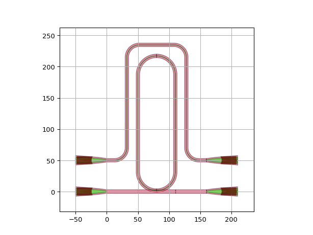
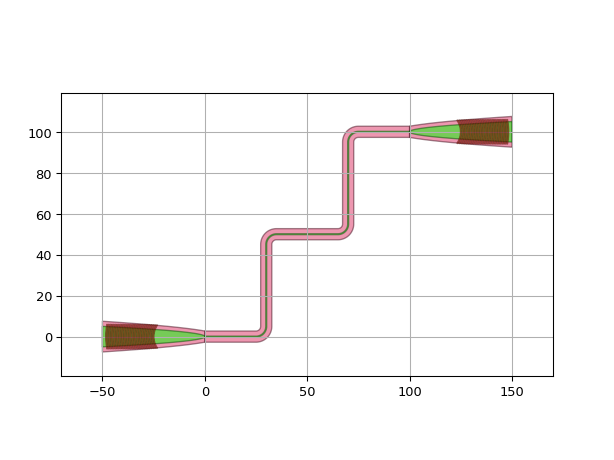
Using Symbols, we can easily route relative to instances or ports:
import si_fab.all as pdk
import ipkiss3.all as i3

gc = pdk.FC_TE_1550()
resonator = pdk.RacetrackResonator(length=500, radius=30)
circuit = i3.Circuit(
    insts={"in1": gc, "in2": gc, "resonator": resonator, "out1": gc, "out2": gc},
    specs=[
        i3.Place("in1:out", (0, 0)),
        i3.Place("in2:out", (0, 50)),
        i3.Place("resonator:in", (50, 0)),
        i3.Place("out1:out", (160, 0), angle=180),
        i3.Place("out2:out", (160, 50), angle=180),
        i3.ConnectManhattan([("in1:out", "resonator:in"), ("resonator:out", "out1:out")]),
        i3.ConnectManhattan(
            "in2:out",
            "out2:out",
            control_points=[
                i3.V(-15, relative_to="resonator@W"),
                i3.H(15, relative_to="resonator@N"),
                i3.V(15, relative_to="resonator@E"),
            ],
            bend_radius=20.0
        ),
    ],
)
circuit.get_default_view(i3.LayoutView).visualize()
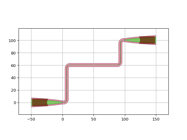
import si_fab.all as pdk
import ipkiss3.all as i3

control_points = [i3.CP((30, 10), i3.NORTH, relative_to=i3.START),  # control point at (30, 10) relative to the start port
                  i3.CP((50, 50), i3.EAST),  # control point at (50, 50) relative to (0, 0)
                  i3.CP((-30, -10), i3.NORTH, relative_to=i3.END)]  # control point at (-30, -10) relative to the end port

gc = pdk.FC_TE_1550()
circuit = i3.Circuit(
    insts={"gc1": gc, "gc2": gc},
    specs=[
        i3.Place("gc1:out", (0, 0)),
        i3.Place("gc2:out", (100, 100), 180),
        i3.ConnectManhattan(
            "gc1:out",
            "gc2:out",
            control_points=control_points,
            bend_radius=5.0
        ),
    ],
)
circuit.get_default_view(i3.LayoutView).visualize()

gc = pdk.FC_TE_1550()
circuit = i3.Circuit(
    insts={"gc1": gc, "gc2": gc},
    specs=[
        i3.Place("gc1:out", (0, 0)),
        i3.Place("gc2:out", (100, 100), 180),
        i3.ConnectManhattan(
            "gc1:out",
            "gc2:out",
            control_points=[i3.H(i3.END - 40)],
            bend_radius=5.0
        ),
    ],
)
circuit.get_default_view(i3.LayoutView).visualize()
Electrical routing
Place a via and change trace template at a certain point along the route. |
In contrast to optical ports, electrical ports typically don’t have a specified angle.
Therefore, routing from one electrical port to another often requires that the start and end angle of the route be determined by the user.
There is also a specialized control point, i3.VIA, that allows you to switch layers and insert vias along the route.
i3.ConnectElectrical is similar to i3.ConnectManhattan but allows us to specify the start_angle and the end_angle when necessary.
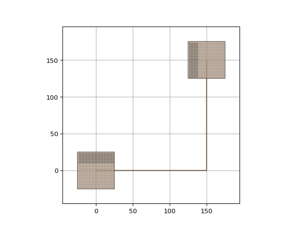
import si_fab.all as pdk  # noqa
import ipkiss3.all as i3

bp = pdk.BondPad()
circuit = i3.Circuit(
    insts={"pad1": bp, "pad2": bp},
    specs=[
        i3.Place("pad1:m1", (0, 0)),
        i3.Place("pad2:m1", (150, 150)),
        i3.ConnectElectrical(
            "pad1:m1",
            "pad2:m1",
            start_angle=0,
            end_angle=-90,
        ),
    ],
)
circuit.get_default_view(i3.LayoutView).visualize()
However, if the angle information is available on the port, then it is not required to specify the corresponding start_angle or end_angle:
import si_fab.all as pdk  # noqa
import ipkiss3.all as i3

class Pad(i3.PCell):
    class Layout(i3.LayoutView):
        size = i3.Size2Property(default=(50.0, 50.0), doc="Size of the bondpad")
        metal_layer = i3.LayerProperty(default=i3.TECH.PPLAYER.M1.LINE, doc="Metal used for the bondpad")

        def _generate_elements(self, elems):
            elems += i3.Rectangle(layer=self.metal_layer, box_size=self.size)
            return elems

        def _generate_ports(self, ports):
            ports += i3.ElectricalPort(
                name="m1",
                position=(0.0, 0.0),
                shape=i3.ShapeRectangle(box_size=self.size),
                process=self.metal_layer.process,
                angle=0,
            )
            return ports

pad = Pad()
M1_wire_tpl = pdk.M1WireTemplate().Layout(width=10)
circuit = i3.Circuit(
    insts={"pad1": pad, "pad2": pad},
    specs=[
        i3.Place("pad1:m1", (0, 0)),
        i3.Place("pad2:m1", (150, 150)),
        i3.ConnectElectrical(
            "pad1:m1",
            "pad2:m1",
            trace_template=M1_wire_tpl,
        ),
    ],
)
circuit.get_default_view(i3.LayoutView).visualize()
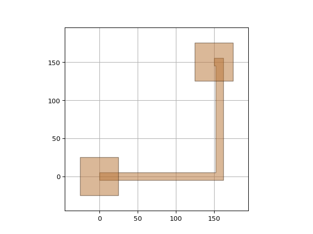
The given start_angle or end_angle will take precedence over the angle of the start or end port:
M1_wire_tpl = pdk.M1WireTemplate().Layout(width=10)
circuit = i3.Circuit(
    insts={"pad1": Pad(), "pad2": Pad()},
    specs=[
        i3.Place("pad1:m1", (0, 0)),
        i3.Place("pad2:m1", (150, 150)),
        i3.ConnectElectrical(
            "pad1:m1",
            "pad2:m1",
            trace_template=M1_wire_tpl,
            end_angle=-90,
        ),
    ],
)
circuit.get_default_view(i3.LayoutView).visualize()

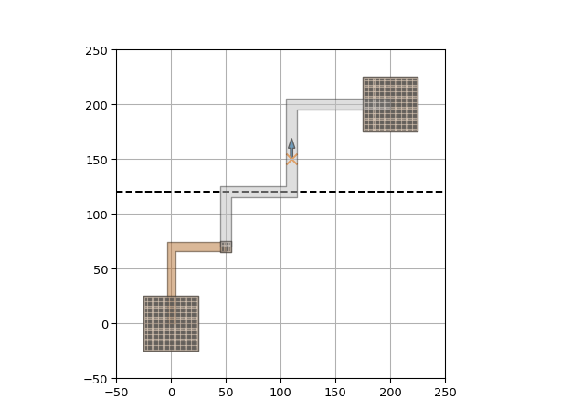
Use i3.VIA and i3.CP to route electrical wire:
import si_fab.all as pdk
import ipkiss3.all as i3
import matplotlib.pyplot as plt

class VIA_M1_M2_ARRAY(i3.PCell):
    box_size = i3.Size2Property(default=(10, 10))
    via_pitch = i3.Size2Property(
        default=i3.TECH.BONDPAD.VIA_PITCH, doc="2D pitch (center-to-center) of the vias"
    )
    via = i3.ChildCellProperty( doc="Via used")

    def _default_via(self):
        return pdk.VIA_M1_M2()

    class Layout(i3.LayoutView):
        def _generate_elements(self, elems):
            elems += i3.Rectangle(layer=i3.TECH.PPLAYER.M1, box_size=self.box_size)
            elems += i3.Rectangle(layer=i3.TECH.PPLAYER.M2, box_size=self.box_size)
            return elems

        def _generate_instances(self, insts):
            periods_x = int(self.box_size[0] / self.via_pitch[0]) - 1
            periods_y = int(self.box_size[1] / self.via_pitch[1]) - 1

            insts += i3.ARef(
                reference=self.via,
                origin=(
                    -(periods_x - 1) * self.via_pitch[0] / 2.0,
                    -(periods_y - 1) * self.via_pitch[1] / 2.0,
                ),
                period=self.via_pitch,
                n_o_periods=(periods_x, periods_y),
            )
            return insts


bp = pdk.BondPad()
via_array = VIA_M1_M2_ARRAY()
M1_wire_tpl = pdk.M1WireTemplate().Layout(width=8)
M2_wire_tpl = pdk.M2WireTemplate().Layout(width=10)

circuit = i3.Circuit(
    insts={"pad1": bp, "pad2": bp},
    specs=[
        i3.Place("pad1", (0, 0)),
        i3.Place("pad2", (200, 200)),
        i3.ConnectElectrical(
            "pad1:m1",
            "pad2:m2",
            start_angle=90,
            end_angle=180,
            trace_template=M1_wire_tpl,
            control_points=[
                i3.VIA(
                    (50, 70),
                    direction_in=i3.WEST,
                    direction_out=i3.NORTH,
                    trace_template=M2_wire_tpl,
                    layout=via_array,
                ),
                i3.CP((None,120)),
                i3.CP((110,150),i3.NORTH)
            ],
        ),
    ],
)
circuit.Layout().visualize(show=False)

plt.axhline(y=120, color='k', linestyle='--')
plt.arrow(110, 150, 0, 10, width=2)
plt.scatter(110,150, c="C1", s=80, marker="x")
plt.show()
Which spec is best for my use-case?
You might be wondering which spec of the above listed better suits your needs, as the same end result can be achieved in various ways. This is why we compiled a small summary that would help you decide:
Placement
Basic
Absolute placement
Multiple position selectors for the instances can be given in the place and route engine:
i3.Place("inst1", (0, 0), angle=45) # angles are always absolute
i3.Place("inst2:port", (0,0), angle=60) # port placement => angle is port angle
i3.Place("inst3@NE", (0,0), angle=45) # the North East corner of the bounding box around the rotated instance will be at (0,0), other (point-like) position selectors are NW, SE, SW, C (for center).
Relative placement
Relative to 1 other thing:
i3.Place("inst1", (10, 10), angle=45, relative_to="inst2:port")
Relative to 2 things, for X and Y separately:
i3.Place("inst1", (10, 10), angle=45, relative_to=("inst2:port", "inst3@NE")) # We take the X value of inst2:port and the Y value of inst3@NE, to calculate the relative placement.
# inst2:port can in this case also be "inst2@E" or "inst2@W", and inst3@NE can be "inst3@N" or "inst3@S", as these are line-like anchors.
Note
Rotation is always absolute, even with relative placement.
Note
i3.Place only works with point-like position selectors/anchors. For line-like position selectors/anchors see below.
Advanced
For the case where you want to place one instance, but want to place/rotate multiple anchors of that one instance: If you want to place the east of the 45 degree rotated instance at X=10, and the port of the instance at Y=5:
i3.Place.X("inst@E", 10) # can also be placed relative_to something else e.g. i3.Place.X("inst@E", 10, relative_to="inst3@W")
i3.Place.Y("inst:port", 5) # can also be placed relative_to something else
i3.Place.Angle("inst", 45)
Note
The position selectors for i3.Place.X and i3.Place.Y can be point-like (in which we take the corresponding value) or line-like (as long as the value corresponds correctly).
Note
i3.Place.X and i3.Place.Y work great together with i3.AlignH, and i3.AlignV respectively.
Routing
Routing can be controlled by passing control_points to your connector, as described in Route control. Control points accept the same types of selector as routing:
i3.ConnectManhattan(
    'grb1:out', 'grb2:out',
    control_points=[
        i3.CP((5, 0), i3.SOUTH, relative_to="inst2:port"), # would pass 5 um to the south from the coordinate of inst2:port
        i3.H(10, relative_to="inst2@N"), # would pass 10 um to north from the north edge of the bounding box of inst2
        i3.V(3, relative_to="inst2@W"), # would pass 3 um to east from the west edge of the bounding box of inst2
        i3.CP((0, -5), relative_to=("inst2@C", "inst2@S")), # would pass through the geometric center of inst2 in the X direction and 5 um to south from the south edge of the bounding box of inst2
    ]
)
Advanced routing with shapes
If the routing specifications are not sufficient for your need and you would like directly control the shape of your routes, have a look at the Routing shapes. Note that the connectors, as a result of providing routing specification, are a layer of functionality on top of the routing shapes.