Rounding algorithms
Rounding algorithms are used in waveguide routing to specify which type of bends to make. The IPKISS waveguides and connectors have a rounding_algorithm parameter which you can set to one of the following:
Returns a shape with circular rounded corners based on a given shape. |
|
Spline based rounding algorithm that is an extension of i3.ShapeRound, used to create adiabatic spline bends. |
|
Euler rounding algorithm that is an extension of i3.ShapeRound, used to create (partial) Euler bends. |
Under the hood, the rounding algorithms are more generic ShapeModifiers, see shape modifier.
Based on the technology that you use, various rounding algorithms might be better suited than the default circular rounding algorithm (ShapeRound).
In the following example, we explain how to use the rounding algorithms to modify an existing shape. There are currently 3 different options. We can create:
circular bends with
ShapeRound,(Bézier) spline bends with
SplineRoundingAlgorithm,Euler bends with
EulerRoundingAlgorithm.
Each of those rounding algorithms take a bend_radius parameter.
For a circular bend this is the constant radius.
For the spline bend, this is the minimum radius: the radius of the circular part or the minimum radius in case the spline covers the full bend.
For the Euler bend, this is the minimum radius as well, unless its use_effective_radius parameter is set, in which case
bend_radiusis interpreted as the effective radius instead.
import ipkiss3.all as i3
import matplotlib.pyplot as plt
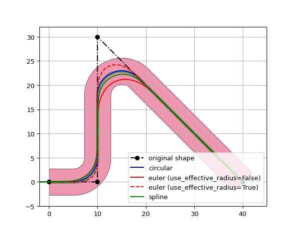
shape = i3.Shape([(0.0, 0.0), (10.0, 0.0), (10.0, 30.0), (40.0, 0.0)])
ra_euler = i3.EulerRoundingAlgorithm(p=0.8)
ra_euler_eff = i3.EulerRoundingAlgorithm(p=0.8, use_effective_radius=True)
ra_spline = i3.SplineRoundingAlgorithm(adiabatic_angles=(20, 20))
shape_circular = i3.ShapeRound(original_shape=shape, radius=5.0)
shape_euler = ra_euler(original_shape=shape, radius=5.0)
shape_euler_eff = ra_euler_eff(original_shape=shape, radius=5.0)
shape_spline = ra_spline(original_shape=shape, radius=5.0)
i3.Waveguide().Layout(shape=shape_circular).visualize(show=False)
plt.plot(shape.x_coords(), shape.y_coords(), 'ko-.', label='original shape')
plt.plot(shape_circular.x_coords(), shape_circular.y_coords(), 'b-', label='circular')
plt.plot(shape_euler.x_coords(), shape_euler.y_coords(), 'r-', label='euler (use_effective_radius=False)')
plt.plot(shape_euler_eff.x_coords(), shape_euler_eff.y_coords(), 'r--', label='euler (use_effective_radius=True)')
plt.plot(shape_spline.x_coords(), shape_spline.y_coords(), 'g-', label='spline')
plt.legend()
plt.xlim(-2, 45)
plt.ylim(-5, 32)
plt.show()
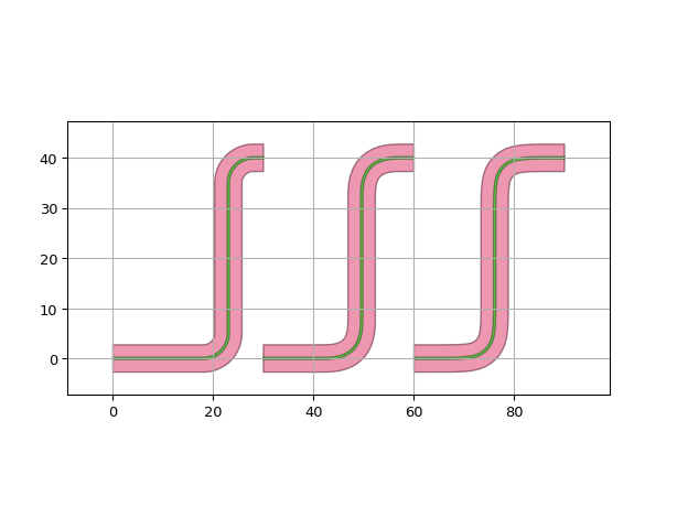
Rounding algorithms in Connectors
The rounding algorithms can be used directly in Connectors such as i3.ConnectBend, as seen below.
p1 = i3.OpticalPort(name="p1", position=(0, 0), angle=0)
p2 = i3.OpticalPort(name="p2", position=(40, 40), angle=180)
p3 = i3.OpticalPort(name="p3", position=(20, 0), angle=0)
p4 = i3.OpticalPort(name="p4", position=(60, 40), angle=180)
p5 = i3.OpticalPort(name="p5", position=(40, 0), angle=0)
p6 = i3.OpticalPort(name="p6", position=(80, 40), angle=180)

c = i3.Circuit(
    specs=[
        i3.ConnectBend(p1, p2, rounding_algorithm=i3.ShapeRound),
        i3.ConnectBend(p3, p4, rounding_algorithm=i3.EulerRoundingAlgorithm(p=0.8)),
        i3.ConnectBend(p5, p6, rounding_algorithm=i3.SplineRoundingAlgorithm(adiabatic_angles=(20, 20))),
    ]
)

c.get_default_view(i3.LayoutView).visualize()
Rounding algorithms in routing functions and RoundedWaveguide
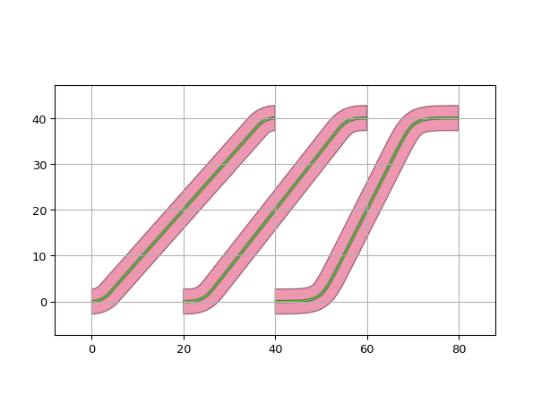
The rounding algorithms can be used directly in Routing functions such as RouteManhattan.
The created route can then be used to create a RoundedWaveguide with the corresponding rounding algorithm for each corner of the route, as seen below:
p1 = i3.OpticalPort(name="p1", position=(0, 0), angle=0)
p2 = i3.OpticalPort(name="p2", position=(30, 40), angle=180)
p3 = i3.OpticalPort(name="p3", position=(30, 0), angle=0)
p4 = i3.OpticalPort(name="p4", position=(60, 40), angle=180)
p5 = i3.OpticalPort(name="p5", position=(60, 0), angle=0)
p6 = i3.OpticalPort(name="p6", position=(90, 40), angle=180)

euler_ra = i3.EulerRoundingAlgorithm(p=0.8)
spline_ra = i3.SplineRoundingAlgorithm(adiabatic_angles=(20, 20))

# a route is a Shape, so we can use it to draw a waveguide
route_circle = i3.RouteManhattan(start_port=p1, end_port=p2)  # Default is ShapeRound
route_euler = i3.RouteManhattan(start_port=p3, end_port=p4, rounding_algorithm=euler_ra)
route_spline = i3.RouteManhattan(start_port=p5, end_port=p6, rounding_algorithm=spline_ra)

# In the Layout of the RoundedWaveguide, you need to specify the rounding algorithm for each corner
wg_circ = i3.RoundedWaveguide().Layout(shape=route_circle)
wg_euler = i3.RoundedWaveguide().Layout(shape=route_euler, rounding_algorithms=[euler_ra, euler_ra])
wg_spline = i3.RoundedWaveguide().Layout(shape=route_spline, rounding_algorithms=[spline_ra, spline_ra])

i3.Circuit(
    insts={
        "wg_circ": wg_circ,
        "wg_euler": wg_euler,
        "wg_spline": wg_spline,
    }
).get_default_view(i3.LayoutView).visualize()
SplineRoundingAlgorithm
- class ipkiss3.all.SplineRoundingAlgorithm
Spline based rounding algorithm that is an extension of i3.ShapeRound, used to create adiabatic spline bends.
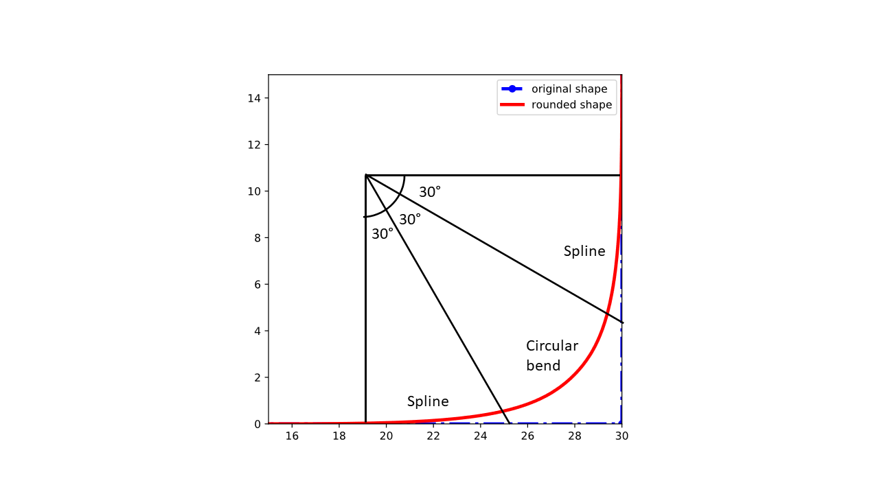
An adiabatic angle is the part of the bend arc over which the bend curvature is gradually increasing from zero (the straight waveguide it connects to) to the required curvature (1/bend_radius).
For example, using SplineRoundingAlgorithm((30,30)) on a 90 degree bend results in the first 30 degrees being covered with a spline, then 30 degrees with a circular bend (constant curvature 1/bend_radius) and then again 30 degrees with a spline.
- Parameters:
- adiabatic_angles: tuple2, optional
Examples
import ipkiss3.all as i3
import matplotlib.pyplot as plt

shape = i3.Shape([(0.0, 0.0), (30.0, 0.0), (30.0, 30.0)])
ra = i3.SplineRoundingAlgorithm(adiabatic_angles=(30, 30))
rounded_shape = ra(original_shape=shape, radius=5.)

plt.figure()
plt.plot(shape.x_coords(), shape.y_coords(), 'bo-.', label='original shape')
plt.plot(rounded_shape.x_coords(), rounded_shape.y_coords(), 'r-', label='rounded shape')
plt.legend()
plt.show()
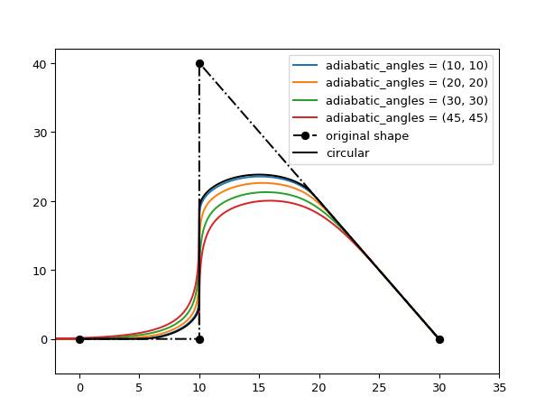
import ipkiss3.all as i3
import matplotlib.pyplot as plt

shape = i3.Shape([(0.0, 0.0), (10.0, 0.0), (10.0, 40.0), (30.0, 0.0)])
shape_circular = i3.ShapeRound(original_shape=shape, radius=5.0)

for angle in [10, 20, 30, 45]:
    ra_spline = i3.SplineRoundingAlgorithm(adiabatic_angles=(angle, angle))
    shape_spline = ra_spline(original_shape=shape, radius=5.0)
    plt.plot(shape_spline.x_coords(), shape_spline.y_coords(),
             label="adiabatic_angles = ({a}, {a})".format(a=angle))

plt.plot(shape.x_coords(), shape.y_coords(), 'ko-.', label='original shape')
plt.plot(shape_circular.x_coords(), shape_circular.y_coords(), 'k-', label='circular')
plt.legend()
plt.xlim(-2, 35)
plt.ylim(-5, 42)
plt.show()
EulerRoundingAlgorithm
- class ipkiss3.all.EulerRoundingAlgorithm
Euler rounding algorithm that is an extension of i3.ShapeRound, used to create (partial) Euler bends. The parameter p defines the fraction of the bend having a linearly increasing curvature, where p=0 indicates a fully circular bend, and p=1 indicates a full Euler bend.
For example, EulerRoundingAlgorithm(p=0.5) on a 90 degree bend results in the first 22.5 (=45/2) degrees being an Euler bend, then 45 degrees being a circular bend, and finally another 22.5 (=45/2) degrees being an Euler bend.
The parameter use_effective_radius determines the meaning of the radius parameter. Other rounding algorithms interpret radius to mean the minimum radius of curvature, which is also the default for EulerRoundingAlgorithm, but you can instead use radius as the effective radius of the bend by setting use_effective_radius to True.
- Parameters:
- use_effective_radius: ( bool, bool_ or int ), optional
interpret radius as the effective radius of the bend instead of the minimum radius of curvature
- p: float and fraction, optional
fraction of the bend having a linearly increasing curvature
Notes
For more information on euler bends see [0]
[0]Florian Vogelbacher, Stefan Nevlacsil, Martin Sagmeister, Jochen Kraft, Karl Unterrainer, and Rainer Hainberger, “Analysis of silicon nitride partial Euler waveguide bends,” Opt. Express 27, 31394-31406 (2019). DOI: 10.1364/OE.27.031394
Examples
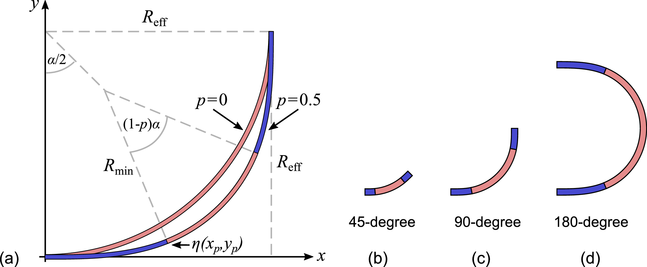
Fig. 1. (a) Geometry of a 90 degree partial Euler bend with bend parameter p=0.5 and a circular bend. The design parameter p influences the angle at which the transition between the section of linearly increasing curvature (blue) to the section with constant curvature (light red) occurs. For p=0 the partial Euler bend is equivalent to a circular bend. The middle section has a radius of curvature of R_min. (b) 45, (c) 90, and (d) 180 degree bend geometries for p=0.2.
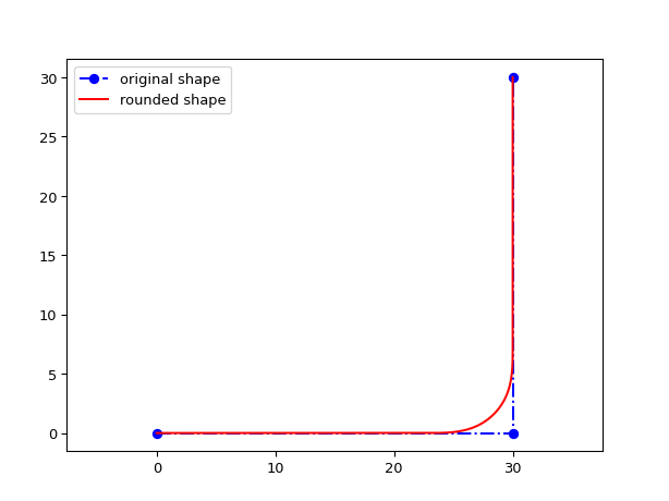
import ipkiss3.all as i3
import matplotlib.pyplot as plt

shape = i3.Shape([(0.0, 0.0), (30.0, 0.0), (30.0, 30.0)])
ra = i3.EulerRoundingAlgorithm(p=0.5)
rounded_shape = ra(original_shape=shape, radius=5.0)

plt.figure()
plt.plot(shape.x_coords(), shape.y_coords(), 'bo-.', label='original shape')
plt.plot(rounded_shape.x_coords(), rounded_shape.y_coords(), 'r-', label='rounded shape')
plt.axis('equal')
plt.legend()
plt.show()
import ipkiss3.all as i3
import matplotlib.pyplot as plt

shape = i3.Shape([(0.0, 0.0), (15.0, 0.0), (15.0, 15.0)])

ra = i3.EulerRoundingAlgorithm(p=1.0)
rounded_shape_euler = ra(original_shape=shape, radius=5.0)

ra_eff_radius = i3.EulerRoundingAlgorithm(p=1.0, use_effective_radius=True)
rounded_shape_euler_eff_radius = ra_eff_radius(original_shape=shape, radius=5.0)

rounded_shape_circular = i3.ShapeRound(original_shape=shape, radius=5.0)

plt.figure()
plt.plot(shape.x_coords(), shape.y_coords(), 'bo-.', label='original shape')
plt.plot(rounded_shape_euler.x_coords(), rounded_shape_euler.y_coords(), 'r-', label='euler rounded shape')
plt.plot(rounded_shape_euler_eff_radius.x_coords(), rounded_shape_euler_eff_radius.y_coords(), 'g-',
         label='euler rounded shape (use_effective_radius=True)')
plt.plot(rounded_shape_circular.x_coords(), rounded_shape_circular.y_coords(), 'y-',
         label='circular rounded shape')

plt.axis('equal')
plt.legend()
plt.show()
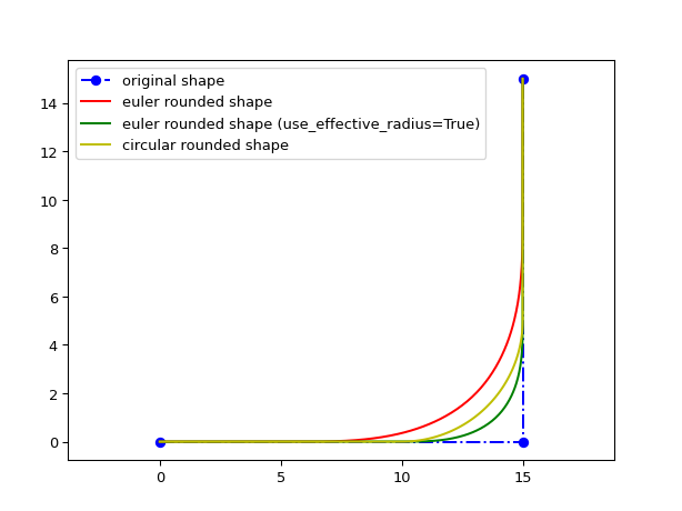
When use_effective_radius is set to True, the radius is the effective radius of the bend (as seen in Figure 1):
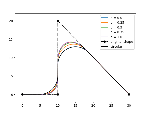
import ipkiss3.all as i3
import matplotlib.pyplot as plt
import numpy as np

shape = i3.Shape([(0.0, 0.0), (10.0, 0.0), (10.0, 20.0), (30.0, 0.0)])
shape_circular = i3.ShapeRound(original_shape=shape, radius=5.0)
for p in np.linspace(0, 1, 5):
    ra_euler = i3.EulerRoundingAlgorithm(p=p, use_effective_radius=True)
    shape_euler = ra_euler(original_shape=shape, radius=5.0)
    plt.plot(shape_euler.x_coords(), shape_euler.y_coords(), label="p = {}".format(p))

plt.plot(shape.x_coords(), shape.y_coords(), 'ko-.', label='original shape')
plt.plot(shape_circular.x_coords(), shape_circular.y_coords(), 'k-', label='circular')
plt.legend()
plt.xlim(-2, 32)
plt.ylim(-2, 22)
plt.show()